This article is Part 1 in a 3-Part Tensorflow 2.0.
Introduction
Tensorflow 2.0 brings a lot of features for rapid development and debugging with eager execution enabled by default. This means that we can run each line of code step by step and immediately see the output of various operations. In previous versions, we had to define all our operations, then create a session to run those operations. There was support for eager execution but it was disabled by default.
In this post, we’ll see how we can create a simple linear regression model and and train this model using gradient descent.
Installtion
First let’s install the library. If you do not have gpu then remove the -gpu.
pip install tensorflow-gpu==2.0.0-beta1
Linear Model
These are the three libraries that we need to import.
1
2
3
import tensorflow as tf
import numpy as np
import matplotlib.pyplot as plt
Now let’s define a linear regression model. We know that a linear model is y = mx + c where m is the slope of the line and c is intercept. So the parameters of this model are m and c. In deep learning terms, we can call them as weight and bias respectively.
So let’s define our model.
1
2
3
4
5
6
7
class Model:
    def __init__(self):
        self.W = tf.Variable(16.0)
        self.b = tf.Variable(10.0)

    def __call__(self, x):
        return self.W * x + self.b
The model above has W and b attributes which will represent the slope and intercept respectively. In the code above, the initial value has ben set to 16 and 10 but in practice they are initialized randomly. In tensorflow, anything that a model learns is defined using tf.Variable. This means that through out the execution, the values of these variables will change i.e. they are mutable.
Next, we define the operation of our model in the __call__ function which accepts an input x. Similar to our equation above, we multiply the input by the weight W and add the bias b. Or in linear regression lingo, we multiply the input by slope and add the intercept.
Note that __call__ is a special function in Python that allows us to treat an object like a function as we’ll see below.
1
2
model = Model()
model(20)
We instantiated our model, and then passed a value 20. Because we implemented __call__ function, we can treat the object like a function. And as expected, we get 330.
1
<tf.Tensor: id=2652, shape=(), dtype=float32, numpy=330.0>
Because of eager execution, we can immediately see the results. The result of the model is a tensor which has no shape i.e. it is a scalar with type float32. In tf2, we can easily convert back and forth between numpy and tensorflow’s tensor objects. As seen above, the tensor also has a numpy value of 330.0. If we want to get the numpy value out of a tensor, we can call numpy() function on a tensor object.
For this demo, let’s create a synthetic dataset. We’ll generate the data such that the slope of the line is 3.0 and intercept is 0.5. We have initialized the model with very different slope and intercept and if our model learns anything, then it should finally figure out that the slope is 3.0 and bias is 0.5.
We sample X i.e. the inputs, from a normal distribution, and some noise as well. Then we generate the y i.e. the outputs using the linear regression formula we saw above.
1
2
3
4
5
6
7
8
TRUE_W = 3.0 # slope
TRUE_b = 0.5 # intercept

NUM_EXAMPLES = 1000

X = tf.random.normal(shape=(NUM_EXAMPLES,))
noise = tf.random.normal(shape=(NUM_EXAMPLES,))
y = X * TRUE_W + TRUE_b + noise
Let’s plot the data as well as the prediction from our untrained model.
1
2
3
plt.scatter(X, y, label="true")
plt.scatter(X, model(X), label="predicted")
plt.legend()
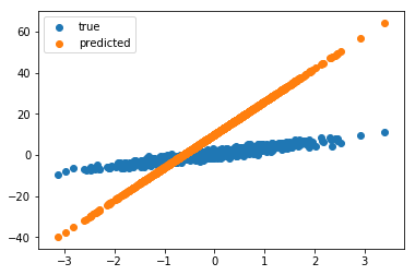
Clearly our model is way off. So we need to train the model. Let’s define a loss function that will tell how bad the model is. We’ll use mean squared error as our loss function.
1
2
def loss(y, y_pred):
    return tf.reduce_mean(tf.square(y - y_pred))
Now, we need to implement a function that will compute the gradient of the model parameters with respect to the loss. Here, we use GradientTape to keep track of operations for the parameters so that we can compute the gradients. Once we get the gradients (using t.gradient function) of W and b patermeters of our model w.r.t the loss, we multiply the gradient with a learning rate and subtract this result from the current value of our parameters (W and b).
1
2
3
4
5
6
7
def train(model, X, y, lr=0.01):
    with tf.GradientTape() as t:
        current_loss = loss(y, model(X))

    dW, db = t.gradient(current_loss, [model.W, model.b])
    model.W.assign_sub(lr * dW)
    model.b.assign_sub(lr * db)
Finally, we define a training loop which updates the weights and biases and also keeps track of the W and b.
1
2
3
4
5
6
7
8
9
10
11
12
13
14
15
16
model = Model()
Ws, bs = [], []
epochs = 20
for epoch in range(epochs):
Ws.append(model.W.numpy()) # eager execution allows us to do this
bs.append(model.b.numpy())
current_loss = loss(y, model(X))
train(model, X, y, lr=0.1)
print(f"Epoch {epoch}: Loss: {current_loss.numpy()}")
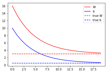
plt.plot(range(epochs), Ws, 'r', range(epochs), bs, 'b')
plt.plot([TRUE_W] * epochs, 'r--', [TRUE_b] * epochs, 'b--')
plt.legend(['W', 'b', 'true W', 'true b'])
plt.show()
The figure below shows that the model was able to figure out the W and b should be around 3.0 and 0.5 respectively.
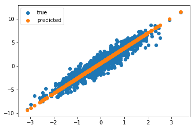
Now if we plot the results from our trained model, we see that the results are much better.
1
2
3
plt.scatter(X, y, label="true")
plt.scatter(X, model(X), label="predicted")
plt.legend()
Conclusion
This post showed a simple linear regression model while taking advantage of eager execution. We also implemented our own “optimizer” using GradientTape.
This article is Part 1 in a 3-Part Tensorflow 2.0.


Comments