Gradient Descent Algorithm From Scratch

Introduction

In this post, we’ll explore Gradient Descent Algorithm and how it is used to train machine learning models. We will implement this algorithm from scratch for a simple linear regression model and compare our implementation against scikit-learn and pytorch implementation. Even though I’ve chosen linear regression model, the concept of gradient descent applies to any kind of model and another reason it to visualize gradient descent in action! Check the video below.

Gradient Descent Algorithm is an optimization algorithm. It tries to find the best values for the parameters of a machine learning model given the learning objectives. In this post, we’ll focus on its application in Machine Learning.

Definitions

Let’s first define few things before we proceed in simple terms. In the later sections, we’ll make these concepts concrete.

Model

First, we will need a model to make predictions. Machine learning model such as linear regression or a deep neural networks are some common examples.

Model parameters

Model parameters are values that a model uses to make predictions. These parameters are initialized randomly before training and the final values are learned during the training. For example, in a linear regression model with single input variable and single output variable, the parameters of this model are \(m\), which indicates slope, and \(c\) which indicates intercept. These parameters are used together to produce the output.

For neural networks, these parameters are also called weights and biases.

Loss function

We need some way to tell if a model is performing better. Also called cost function or objective function, it gives lower values when a model performs better.

Typical examples of loss functions used in practice are

• Mean Squared Error: When the output is a numerical value, this loss function is common choice
• Binary Cross Entropy: It is used when we want to do binary classification e.g. will it rain or not, is it a cat or a dog, has disease or no disease
• Categorical Cross Entropy: It is used when we want to do multi-class classification e.g. predict the category of new articles from 10 possible categories.

Deep dive

Let’s explore this algorithm with concrete example to make it clear. First we’ll need a model to begin with. Will consider a simple linear regression model with one input and one output. In this case our model has two parameters \(m\), a slope, and \(c\), an intercept. These two parameters are used in the model in the following way: \(y = mx + c\)

Model

Linear regression is a method used to find a linear equation that best predicts the output using the input variables.

The equations for a case where there is only a single input variable is as follows

\[y = mx + c\]

Where,

• \(y\) is the output
• \(x\) is the input variable
• \(m\) is the slope of the line
• \(c\) is the intercept

\(m\) and \(c\) are parameters of the model. In this case, we can say that this model has 2 parameters. Compare this with ChatGPT, which is rumored to have around 175 billion parameters.

The implementation is quite simple for a linear regression model since in our case, we only have one input variable. This function accepts slope, intercept and the input data X as parameters and computes the prediction based on the forumla \(y = mx + c\).

def linear_regression(slope, intercept, X):
    return slope * X + intercept

Loss function

For our linear regression model which values for the parameters slope and intercept should we use? Is using 0.5 as slope better than 3.7?. This is where loss functions come in.

Loss function gives lower value when the predicted values closely match the true outputs.

Therefore, when the loss function’s value is minimized, it means that the model parameters, in this case slope and intercept, are tuned to ensure predictions from model closely match the true outputs.

Since our output is a numerical value, we will use Mean Squared Error as our loss function.

The implementation is fairly straight forward, we first compute the difference between true output and predicted output and then square it and then compute the mean of these differences. Note that y_true and y_pred are numpy arrays rather than a single numbers.

def mse(y_true, y_pred):
    return ((y_true - y_pred)**2).mean()

The animation below shows MSE in action. The table on the right shows the ground truth and the predicted values. Notice as the predicted values are closer to the ground truth, the loss value decreases.

Data exploration

To train this model, let’s create a toy dataset.

from sklearn.datasets import make_regression
from sklearn.model_selection import train_test_split

X, y, true_slope = make_regression(
    n_samples=100,
    n_features=1,
    n_informative=1,
    n_targets=1,
    noise=5,
    coef=True,
    random_state=2,
)

X_train, X_test, y_train, y_test = train_test_split(X, y, test_size=0.2)

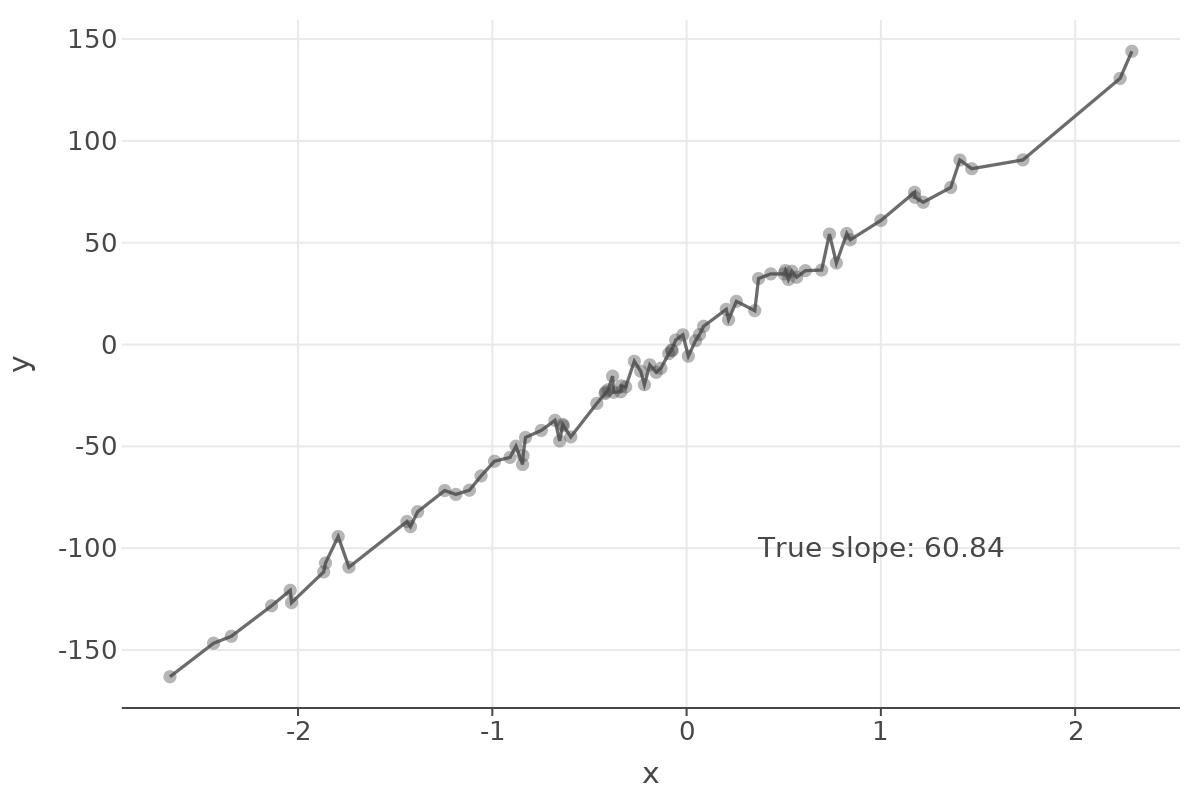
When we plot the input in x-axis and the output in y-axis, we see that as the input value increases, the output also increases. If we look that the “true slope” value used by scikit-learn to generate this data, we see the value is 60.84, this means if the input is increased by 1, then the output will increase by 60.84.

Gradient Descent

Ok, so far we have the model and the loss function defined. But how do we find the best values for the model parameters so that the predictions are close to the true outputs.

We know that we need to minimize the loss. How do we do this?

First, we need to compute the gradient of the loss function with respect to each parameter in our model.

Gradient is basically a list of partial derivatives of loss function with respect to reach parameter. Gradient can be thought as a a vector indicating the direction of steepest ascent in the loss surface.

Since we want to go towards the direction where the loss is minimized, we will go in the opposite direction indicated the gradient.

Here we have two parameters, so we need to find two partial derivatives. If your calculus skills is rusty, you can use sympy library to calculate the derivaties for you as well. Note that when using libraries like Pytorch or Tensorflow, we do not need to calculate the derivatives ourselves. It is done by the library automatically!

import sympy
x, slope, intercept = sympy.symbols("x, slope, intercept")
y_true = sympy.symbols("y_true", constant=True)
y_pred = slope * x + intercept
loss = (y_true - y_pred)**2
display(loss.diff(slope).simplify())
display(loss.diff(intercept).simplify())

The partial derivative of the loss function with respect the the slope is \(-2x(y_{true} - y_{pred})\).

Similarly, the partial derivative of the loss function with respect to the intercept is \(-2(y_{true} - y_{pred})\).

Now that we know the gradient, we use the following rule to update the values of parameters so that we move in the direction where loss is minimized.

\[slope = slope - (lr * \frac{\partial L}{\partial slope})\] \[intercept = intercept - (lr * \frac{\partial L}{\partial intercept})\]

Here learning rate (lr) is hyper-parameter that we have to choose and is usually set between 0 and 1. The learning rate basically scales down the amount we move in the loss surface. Typical values are 0.001 and 0.0001.

We have all the basics needed for implementing gradient descent algorithm. Now let’s look at the code.

def sgd_step(slope, intercept, X, y, lr=0.1):
    y_pred = linear_regression(slope=slope, intercept=intercept, X=X)
    # compute the derivative of loss function wrt. slope
    dl_dslope = -(2 * (y - y_pred) * X).mean()
    # compute the derivative of loss function wrt. intercept
    dl_dintercept = -(2 * (y - y_pred)).mean()

    # update the parameters
    slope = slope - (lr * dl_dslope)
    intercept = intercept - (lr * dl_dintercept)
    return slope, intercept, dl_dslope, dl_dintercept

Here, I’ve defined a function called sgd_step which accepts slope, intercept which are the model paramters and the input X and output y. It also accepts learning rate as lr.

First we compute the predictions using current value of model parameter. Then we compute the partial derivative of loss with respect to slope parameter. Since we are doing this for a batch of data, we take the mean of all derivaties.

Similarly we compute the partial derivative of loss with respect to the intercept paramter.

Next, we update the model parameters using the update rule of Gradient Descent algorithm.

And finally we return the updated slope and intercept values. I’ve returned the partial derivaties for visualization purpose but it is not necessary.

The sgd_step function only updates the model paramters once. But we need to do this many times.

So, here is a complete training procedure.

import toolz

# initialize the parameters to some value
slope = -10
intercept = 9

epochs = 10
bs = 32

def train(slope, intercept, X, y, epochs=10, bs=32, lr=0.1):
    for epoch in range(epochs):
        # split the data into batches
        for batch_ids in toolz.partition_all(
            bs, np.random.permutation(np.arange(len(X)))
        ):
            batch_ids = np.array(batch_ids)
            batch_x = X[batch_ids]
            batch_y = y[batch_ids]
            slope, intercept, dl_slope, dl_intercept = sgd_step(
                slope=slope, intercept=intercept, X=batch_x, y=batch_y, lr=lr
            )

        # calculate the loss for this epoch
        # Note: typically losses are collected for each batch in the epoch and then average is taken as loss for the epoch
        loss = mse(y, linear_regression(slope=slope, intercept=intercept, X=X))
        print(f"Loss at epoch {epoch} = {loss}")

    return slope, intercept

# since X_train is a matrix with 1 column, we take all rows and first column as input vector X
slope, intercept = train(
    slope=slope, intercept=intercept, X=X_train[:, 0], y=y_train, lr=0.1
)
print(slope, intercept)
# (60.134316467596285, -0.00922299723642274)

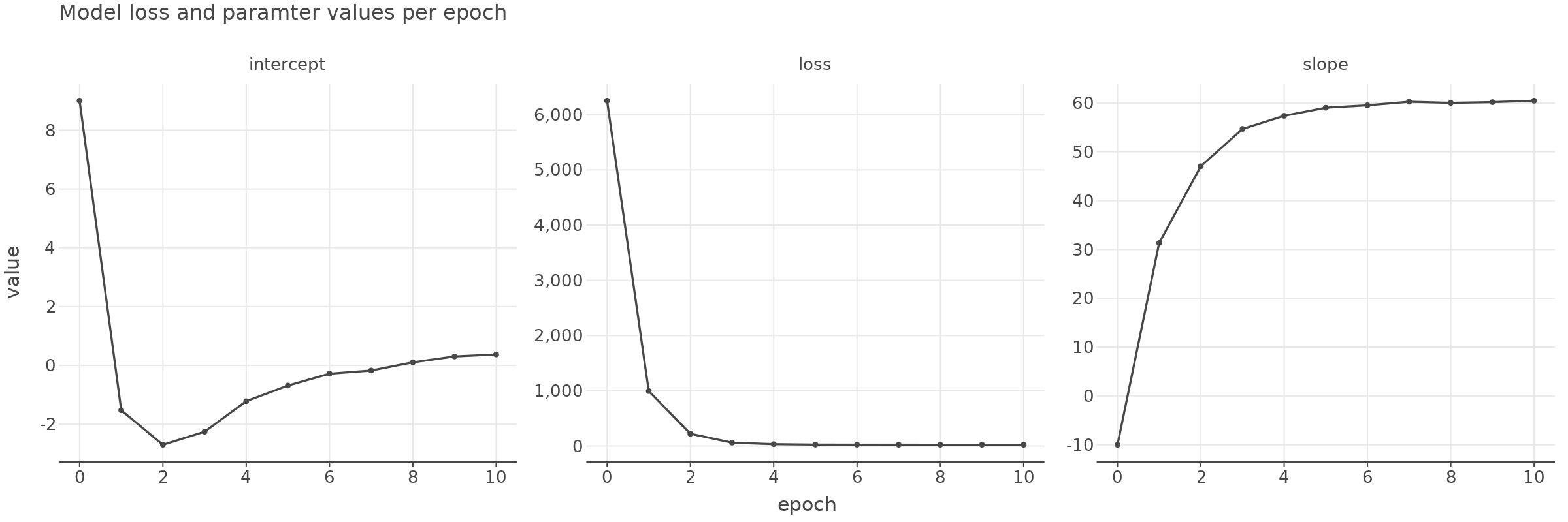
First we randomly initialize our model parameters. Second we define the number of epochs to run. In each epoch, the model will see a complete data set. We need to run this many times so we set the epochs as 10 here.

Third, we set the batch size. For one update of model parameters, we will use that many samples in our dataset. This is the most common approach for training deep neural networks as not all dataset will fit in the memory. This version of Gradient Descent algorithm is also called Gradient Descent with mini-batch.

Then comes the actual training loop. For each epoch, we partition our data into batches. Then call the sgd_step function with this batch of data. We will replace values of slope and intercept with the values returned by the function so that next time it is called, it will use the updated values of these parameters.

If we visualize the loss value and parameter values over each epoch then we can see them converging as the epoch progresses.

Evaluation and comparison with sklearn and pytorch

Now let’s see how does this model work on our test set.

y_pred = linear_regression(slope=slope, intercept=intercept, X=X_test[:, 0])
print("MSE = ", mse(y_test, y_pred))
# MSE =  21.184015118341343

Let’s compare this with sklearn implementation

from sklearn.linear_model import SGDRegressor
lr = SGDRegressor().fit(X_train, y_train)
print(f"Slope = {lr.coef_[0]}, Intercept = {lr.intercept_[0]}")
print("MSE = ", mse(y_test, lr.predict(X_test)))

# Slope = 60.044860375107355, Intercept = -0.0518031540413587
# MSE =  21.320319924030493

Seems pretty close! The parameters found by sklearn and MSE on test data is almost the same as the values we found ourselves.

For one more comparison, let’s implement this using Pytorch and compare against it.

import torch
class TorchLR(torch.nn.Module):
    def __init__(self):
        super().__init__()
        self.slope = torch.nn.Parameter(data=torch.tensor(1.0, dtype=torch.float32), requires_grad=True)
        self.intercept = torch.nn.Parameter(data=torch.tensor(1.0, dtype=torch.float32), requires_grad=True)

    def forward(self, X):
        return X * self.slope + self.intercept
    
torch_lr = TorchLR()
optim = torch.optim.SGD(torch_lr.parameters(), lr=0.1)
loss_fn = torch.nn.MSELoss()
epochs = 10
for epoch in range(epochs):
    for batch_ids in toolz.partition_all(bs, np.random.permutation(np.arange(len(X)))):
        batch_ids = np.array(batch_ids)
        batch_x = torch.tensor(X[batch_ids])
        batch_y = torch.tensor(y[batch_ids])

        optim.zero_grad()
        
        loss_val = loss_fn(batch_y, torch_lr(batch_x[:, 0]))

        # these two steps automatically compute the gradients and perform the parameter updates!!
        # we do not need to calcuate the gradients and do the parameter updates ourselves!!
        # this logic is exactly the same even if our model had millions of parameters.
        loss_val.backward()
        optim.step()

    if epoch % 5 == 0 or epoch == epochs - 1:
        print(f"Epoch {epoch}, Loss = {loss_val}")

print()
print(f"Slope = {torch_lr.slope.data}, intercept = {torch_lr.intercept.data}")
print("MSE = ", mse(y_test, torch_lr(torch.tensor(X_test[:, 0])).detach().numpy()))

# Slope = 59.92798614501953, intercept = 0.7032995223999023
# MSE =  20.868084536438573

Once more, the parameters and the loss values are quite close.

Gradient Descent Visualization

Let’s visualize how the gradient descent algorithm works.

In the right hand side of the plot below, we can see the loss surface where the black color indicates higher loss values and white color indicates lower loss values. For each combination of Intercept and Slope, we can see different loss values.

In the Y-axis, we see the range of values for the intercept parameter which ranges from 10 to -10 in this case.

And similarly in the x-axis, we see the range of values for the slope parameter. Here we see the values range between -100 to 200.

To create this loss surface plot, for each pair of slope and intercept, we calculate the loss value and use contour plot visualize it.

To interpret this plot, lets take an example. When the slope is around 200 or -100, we have higher loss values compared to the cases when the slope is between 0 and 100.

We also know that when slope is at around 60 and intercept is at around 0, we have the lowest loss possible.

In the right hand side, the plot shows the ground truth in light blue color and the model prediction using the current value of slope and intercept parameter. As the parameters change, this line will also get updated.

Effect of Learning Rate

Now, let’s see how the learning rate affects the convergence. In this case, the learning rate is 0.1 and we will let it run for 10 epochs. We can see the algorithm makes small updates in the parameters and ultimately converges to the lowest loss.

When the learning rate is 0.6 (see below), we see it makes bigger updates.

When learning rate is 0.8 (see below), it makes even bigger updates to the parameters and even though it almost found the parameters with lowest loss at around epoch 7, it still kept making bigger changes and kept overshooting the place with lowest loss and did’t converge even up to 50 epochs.

Conclusion

In this post we implemented our own version of gradient descent algorithm for linear regression model. However, the same concept is true for even the most complex deep neural networks! The basic idea is for each parameter of our model, we need to compute the partial derivative of loss function with respect to that parameter and then use the update rule to update the parameter’s value.

With libraries like Pytorch, Tensorflow, JAX etc. we do not even have to compute the gradients since they are automatically calculated by the libraries. However, it is important to understand the idea behind the algorithm which I hope I have helped you understand gradient descent algorithm a bit more than you did before reading this post.

That is all I wanted to share. Please let me know if you find any mistakes in this post. Thanks for reading.