Introduction
In the previous post we used a pre-trained model to extract feature vectors out of images and use K-Nearest Neighbors to find similar images. One issue we have using pre-trained models is that they don’t perform that well on the data it has not seen while training it. So in many cases we need to fine tune the model using our own dataset.
The goal of this post is to compare a pre-trained model vs fine-tuned model for “Image search” problem. Full source code for this post can be found here.
Let’s import the libraries we will use for this demo
1
2
3
4
5
6
import tensorflow as tf
import tensorflow_hub as hub
import tensorflow_datasets as tfds
import numpy as np
import matplotlib.pyplot as plt
import functools
Dataset
We will use oxford_flowers102 dataset which contains 102 flower categories where each class consists 40-250 images. Please check the link for more details. I’ve chosen this dataset because it is relatively small (~350 MB) compared to other data sets available in Tensorflow Datasets catalog. You can also choose to use your own dataset if you prefer.
Also for the purpose of the demo and due to my hardware limitation, I’ve only decided to take examples from the first 20 classes instead of all 102 classes. You can remove the call to filter method of train_ds and valid_ds if you would like to use all available data.
1
2
3
4
5
6
7
8
9
10
11
12
13
14
15
16
17
18
19
20
(train_ds, valid_ds), info = tfds.load("oxford_flowers102", split=["train", "validation"], as_supervised=True, with_info=True)
int_to_class_label = info.features['label'].int2str


CLASSES_TO_CONSIDER = list(range(20)) # only take first 20 classes for demo
IMG_WIDTH = IMG_HEIGHT = 256

def preprocess_image(image, label, height, width):
    image = tf.image.resize_with_crop_or_pad(image, target_height=height, target_width=width)
    image = tf.cast(image, tf.float32) / 255.0
    return image, label

def filter_by_classes(img, label):
    bools = tf.equal(label, CLASSES_TO_CONSIDER)
    return tf.reduce_any(bools)


partial_preprocess_image = functools.partial(preprocess_image, height=IMG_HEIGHT, width=IMG_WIDTH)
train_ds = train_ds.filter(filter_by_classes).map(partial_preprocess_image).cache().shuffle(buffer_size=1000)
valid_ds = valid_ds.filter(filter_by_classes).map(partial_preprocess_image).cache().shuffle(buffer_size=1000)
Also for simplicity and to create a custom batch data generator (which I will explain later), let’s load every thing in memory.
1
2
3
4
5
6
7
8
9
10
11
def get_x_y_from_ds(ds):
    x, y = [], []
    for img, label in ds.cache().as_numpy_iterator():
        x.append(img)
        y.append(label)

    return np.array(x), np.array(y)

x_train, y_train = get_x_y_from_ds(train_ds)
x_test, y_test = get_x_y_from_ds(valid_ds)
print(len(x_train), len(y_train), len(x_test), len(y_test)) # 200 200 200 200
After running that we end up with 200 training samples and 200 testing samples.
Visualize embeddings using Pre-trained model
Let’s extract the feature vectors or embeddings using a pre-trained model and plot the vectors in 2D space. This will give us an idea of how good the model is at generating vectors for images from different categories. Ideally we want images from same class to be very close to each other and as far as possible from images of other classes.
The code below is a helper function that transforms the feature vector to 2D space using TSNE and plots it.
1
2
3
4
5
6
7
8
9
10
11
from sklearn.decomposition import PCA
from sklearn.manifold import TSNE
import plotly.express as px

def plot_embeddings(features, labels):
    pca = TSNE(n_components=2, learning_rate='auto', init='pca')
    reduced_features = pca.fit_transform(features)
    str_labels = list(map(int_to_class_label, labels))
    fig = px.scatter(x=reduced_features[:,0], y=reduced_features[:,1], color=str_labels, symbol=labels)
    fig.show()
Pretrained ResNet 50 model
Let’s use a pretrained model from TFHub called Resnet 50. It has been trained on ImageNet dataset. As far as I’m aware ImageNet dataset does not contain images of flowers so let’s see how well it performs on this new dataset.
1
2
3
4
5
6
MODEL_URL = "https://tfhub.dev/google/imagenet/resnet_v2_50/feature_vector/5"
vectorizer = tf.keras.Sequential([
    hub.KerasLayer(MODEL_URL, trainable=False)
])
vectorizer.build([None, IMG_HEIGHT, IMG_WIDTH, 3])
vectorizer.summary()
This model has around 23 million parameters. let’s extract the feature vectors and plot them.
1
2
pre_trained_features = vectorizer.predict(x_test)
plot_embeddings(features=pre_trained_features, labels=y_test)
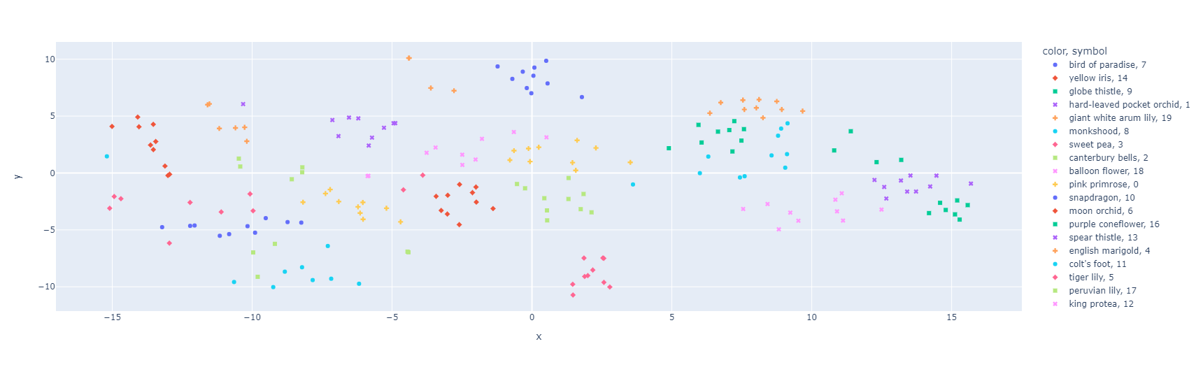
The figure above shows that the datapoints are scattered. Also note that plotly chose to use very similar colors for multiple classes so it might seem they are completely scattered but it is actually not that bad for embeddings from a pre-trained model.
Let’s also write some helper functions to interactively view the similar images using Jupyter widgets.
1
2
3
4
5
6
7
8
9
10
11
12
13
14
15
16
17
18
19
20
21
22
23
24
25
26
27
28
29
30
31
32
33
34
35
from sklearn.neighbors import NearestNeighbors
def get_knn(features):
    knn = NearestNeighbors(n_neighbors=5, metric="cosine")
    knn.fit(features)
    return knn

import ipywidgets as w
def show_similar_images(images, labels, vectorizer, knn, start_image_idx, n_inputs=5, n_neighbors=10):
    input_images = images[start_image_idx:start_image_idx+n_inputs]
    features = vectorizer.predict(input_images)
    knn_output = knn.kneighbors(features, n_neighbors=n_neighbors)

    images_with_distances_and_nbors = zip(input_images, *knn_output)

    fig, axes = plt.subplots(len(input_images), n_neighbors+1, figsize=(20, len(input_images)*4))

    for i, (image, distances, nbors) in enumerate(images_with_distances_and_nbors):
        for j in range(n_neighbors+1):
            ax = axes[i, j]
            img = (image if j==0 else images[nbors[j-1]])
            if j == 0:
                ax.set_title("Input Image")
            else:
                ax.set_title(f"Sim: {1-distances[j-1]:.2f}")
                ax.set_xlabel(f"lbl: {labels[nbors[j-1]]}")
            ax.get_xaxis().set_ticks([])
            ax.get_yaxis().set_ticks([])
            ax.imshow(img)

pretrained_knn = get_knn(features=pre_trained_features)
w.interact(show_similar_images, images=w.fixed(x_test), labels=w.fixed(y_test), vectorizer=w.fixed(vectorizer), knn=w.fixed(pretrained_knn),
    start_image_idx=w.IntSlider(max=len(x_test)-1, continuous_update=False),
    n_inputs=w.IntSlider(min=2, value=5, max=10, continuous_update=False),
    n_neighbors=w.IntSlider(min=2, value=5, max=10, continuous_update=False),
)
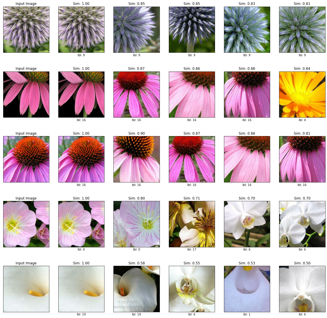
The results look ok. It seems to find images that look similar to the input image. But take a closer look at the labels of the similar images. They are not always from the same class as the input. The first image in the result is the same image as the input image with similarity of 1.0. Ideally we want all results from from the same class. We can improve the results by fine tuning.
Fine tuning using Online Triplet mining
Triplet loss was introduced in the FaceNet paper which forces the neural network to reduce the distance of the embedding vectors from same class while maximizing the distance between embeddings of different classes. You can find more details here and here.
Let’s define our model
1
2
3
4
5
6
7
8
9
10
tuned_vectorizer = tf.keras.Sequential([
    tf.keras.layers.RandomFlip("horizontal_and_vertical"),
    tf.keras.layers.RandomRotation(0.2),
    hub.KerasLayer(MODEL_URL, trainable=True),
    tf.keras.layers.Dropout(0.3),
    tf.keras.layers.Dense(384, activation=None), # No activation on final dense layer
    tf.keras.layers.Lambda(lambda x: tf.math.l2_normalize(x, axis=1)) # L2 normalize embeddings
])
tuned_vectorizer.build([None, IMG_HEIGHT, IMG_WIDTH, 3])
tuned_vectorizer.summary()
We add two layers that augment the data during training process to make sure that the model sees different variation of image while training. These layers are not active during the prediction. The third layer is the pre-trained model from TFHub with trainable=True. After a dropout layer we have a linear layer which outputs 384 dimension vector without any activation. The loss function we are going to use expects L2 normalized embeddings without any activation function like relu applied.
Now that we have the model ready to be trained, we need to give the model some data to train. According to the FaceNet paper:
On all datasets we train using a batch size of 128. Batches are constructed with a fixed number n examples per class by adding classes until the batch is full. When a class has fewer than n examples, we use all the examples from the class. If this leads to a case where the last class in the batch does not have space for n images, we just include enough images to fill the batch
So we need a custom batch generator that implements this logic. I came up with a simple version that I believe does what the authors have mentioned.
1
2
3
4
5
6
7
8
9
10
11
12
13
14
15
16
17
18
19
20
21
from collections import defaultdict
import random

def get_training_batch(images, labels, batch_size=128, n_examples_per_class=3):
    examples_per_class = defaultdict(list)
    for x, y in zip(images, labels):
        examples_per_class[y].append(x)

    while True:
        batch_X, batch_y = [], []
        while len(batch_X) < batch_size:
            for cls, examples in examples_per_class.items():
                n_sample = min(n_examples_per_class, (batch_size - len(batch_X)))
                if n_sample == 0:
                    break
                samples = random.sample(examples, k=n_sample)
                batch_X.extend(samples)
                batch_y.extend([cls] * len(samples))

        yield np.array(batch_X), np.array(batch_y)
Now we are ready to fine tune the model. Before that we need to install tensorflow_addons library using pip install tensorflow_addons. This library has implementation of the loss function we will be using.
1
2
3
4
5
6
7
8
9
10
11
12
13
14
15
16
bs = 64
n_examples_per_class = 3
initial_lr = 0.0001
epochs = 80
import tensorflow_addons as tfa

tuned_vectorizer.compile(optimizer=tf.keras.optimizers.Adam(learning_rate=initial_lr),
                         loss=tfa.losses.TripletSemiHardLoss())

history = tuned_vectorizer.fit(get_training_batch(images=x_train, labels=y_train, batch_size=bs, n_examples_per_class=n_examples_per_class),
                               callbacks=[tf.keras.callbacks.EarlyStopping(patience=5)],
                               epochs=epochs,
                               steps_per_epoch=len(x_train)//bs,
                               validation_data=(x_test, y_test),
                               validation_batch_size=bs,
                              )
While the authors of FaceNet paper mentioned a batch size of 128, due to my hardware limitation I had to set the batch size to 64. Also with some hit and trial, I found best results using n_example_per_class = 3. FaceNet authors also do some analysis on the effect of this parameter in their paper.
The log below shows the output of the training process.
1
2
3
4
5
6
7
8
9
10
Epoch 1/80
3/3 [==============================] - 13s 1s/step - loss: 1.2295 - val_loss: 1.1830
Epoch 2/80
3/3 [==============================] - 3s 1s/step - loss: 1.2226 - val_loss: 1.1624
...
Epoch 60/80
3/3 [==============================] - 3s 1s/step - loss: 0.2685 - val_loss: 0.4850
...
Epoch 80/80
3/3 [==============================] - 3s 1s/step - loss: 0.2559 - val_loss: 0.4574
Visualize embeddings using fine tuned model
Ready for the big moment? Let’s plot the embeddings and see how it looks like.
1
2
frozen_features = tuned_vectorizer.predict(x_test)
plot_embeddings(features=frozen_features, labels=y_test)
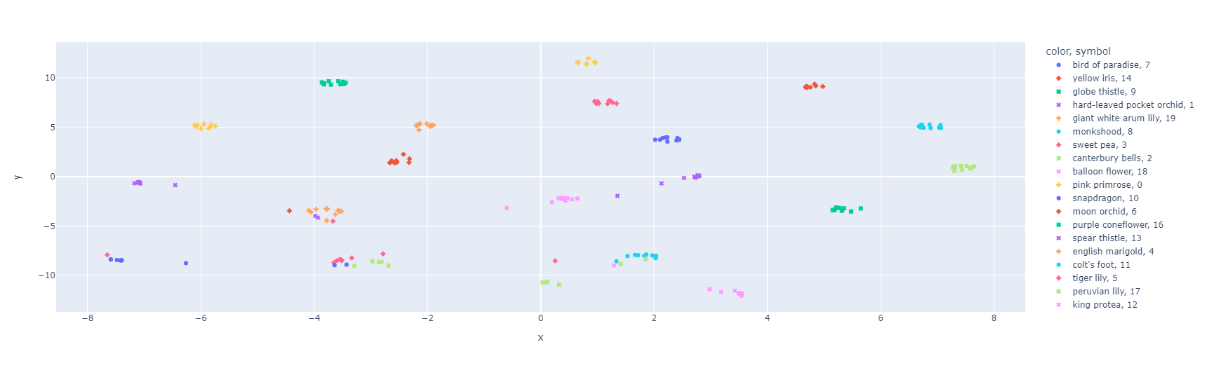
The results look awesome right? It seems almost all of the classes are closely grouped together while being far away from other groups. This is due to the nature of the loss function we used to train the model - reduce the distance of embeddings from same class while maximizing the distance from other classes.
Using our interactive Jupyter widget helper, we can see the results of “Image search”
1
2
3
4
5
6
frozen_knn = get_knn(features=frozen_features)
w.interact(show_similar_images, images=w.fixed(x_test), labels=w.fixed(y_test), vectorizer=w.fixed(tuned_vectorizer), knn=w.fixed(frozen_knn),
    start_image_idx=w.IntSlider(max=len(x_test)-1, continuous_update=False),
    n_inputs=w.IntSlider(min=2, value=5, max=10, continuous_update=False),
    n_neighbors=w.IntSlider(min=2, value=5, max=10, continuous_update=False),
)
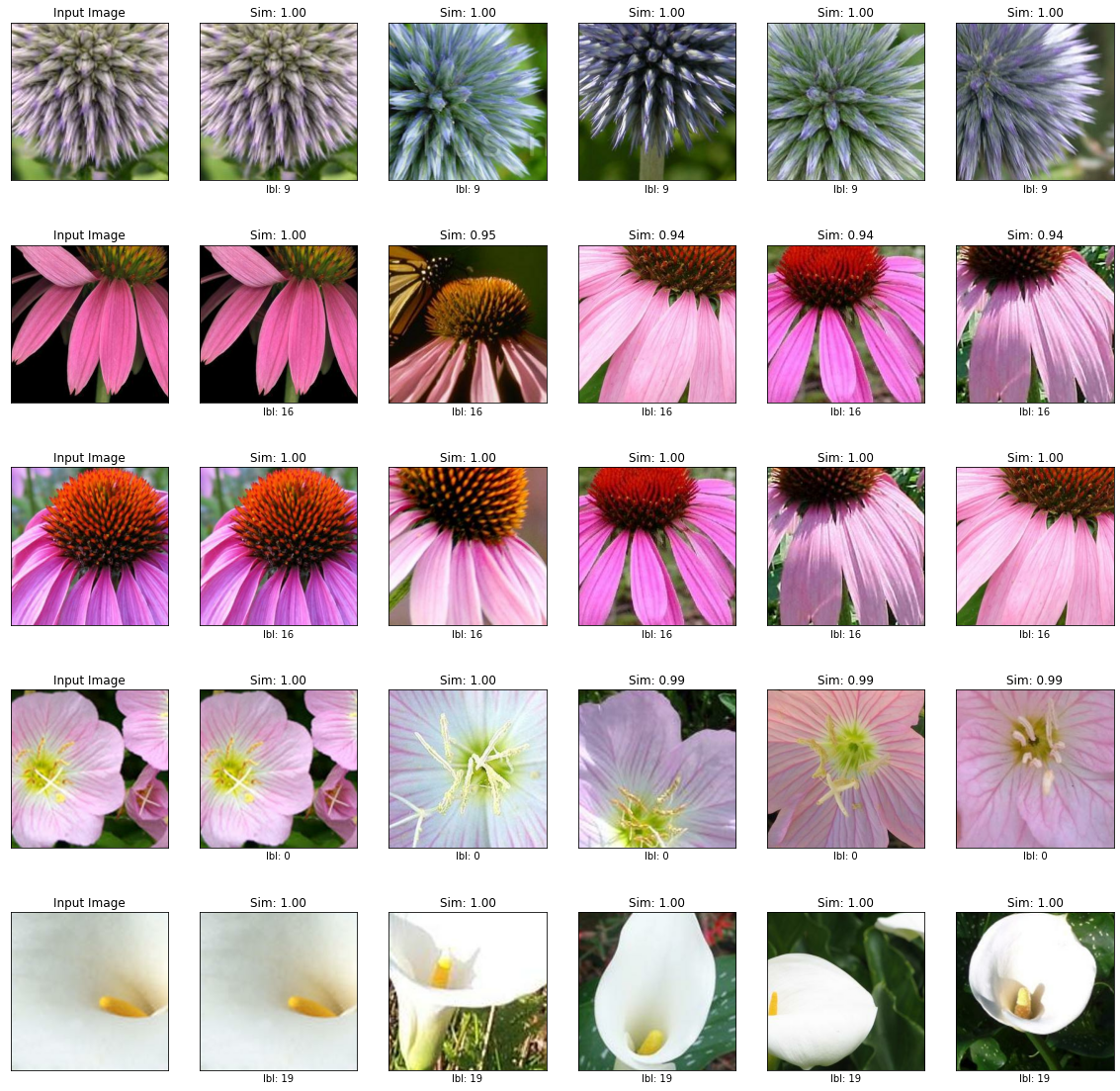
The figure above shows the results for exactly the same inputs as before. All of the results are from the same class as the input image and also note the similarity score - they are close to 1.0.
Conclusion
In this post, we saw how to fine tune a pre-trained ResNet50 model using TripletSemiHardLoss loss function. In the next post we will look at how we can deploy this model into a “Production” grade application.


Comments