This article is Part 2 in a 3-Part Tensorflow 2.0.
Introduction
In this post, we’ll design and train a simple feed-forward neural network to classify images into 1 of 10 labels. We’ll use keras, a high level deep learning library, to define our model and train it. Keras is part of tensorflow library so separate installation is not necessary.
Let’s import the necessary libraries.
1
2
3
4
5
6
7
8
9
10
import math

import tensorflow as tf
from tensorflow import keras

import numpy as np
import matplotlib.pyplot as plt
%matplotlib inline

print(tf.__version__)
2.0.0-beta1
Dataset
We’ll be using FashionMNIST dataset published by Zalando Research which is a bit more difficult than the MNIST hand written dataset. This dataset contains images of clothing items like trousers, coats, bags etc. The dataset consists of 60,000 training images and 10,000 testing images. Each image is a grayscale image with size 28x28 pixels. There are 10 total categories and each label is assigned a number between 0 and 9. Corresponding class labels can be found https://github.com/zalandoresearch/fashion-mnist#labels
Keras already comes with FashionMNIST dataset helper and will download it if it does not already exists in your machine. Let’s load the dataset and explore a bit.
First download and load the dataset
1
2
3
fashion_mnist = keras.datasets.fashion_mnist

(x_train, y_train), (x_test, y_test) = fashion_mnist.load_data()
Let’s check how many samples are there in training and testing set as well their size and also the categories.
1
x_train.shape, x_test.shape, np.unique(y_train)
1
2
3
((60000, 28, 28),
 (10000, 28, 28),
 array([0, 1, 2, 3, 4, 5, 6, 7, 8, 9], dtype=uint8))
The output shows that we have 60K training images, 10K testing images where each image is of size 28x28 pixels. Similarly, the categories are numbers from 0 to 9. The class labels are not particularly helpful so let’s assign human friendly name for each of the labels. Again, you can find the readable labels at https://github.com/zalandoresearch/fashion-mnist#labels
1
2
 class_names = {i:cn for i, cn in enumerate(['T-shirt/top', 'Trouser', 'Pullover', 'Dress', 'Coat',
               'Sandal', 'Shirt', 'Sneaker', 'Bag', 'Ankle boot']) }
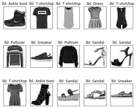
Let’s plot some images and their labels and check our dataset.
1
2
3
4
5
6
7
8
9
10
11
12
13
14
15
16
17
18
19
20
21
22
23
24
25
26
27
28
29
30
 def plot(images, labels, predictions=None):
    """Helper function to plot images, labels and predictions
    Parameters
    ----------
    images : 3D matrix of image
    labels : 1D array
    predictions (optional): 1D array
    """
    # create a grid with 5 columns
    n_cols = min(5, len(images))
    n_rows = math.ceil(len(images) / n_cols)
    fig, axes = plt.subplots(n_rows, n_cols, figsize=(n_cols+3, n_rows+4))

    if predictions is None:
        predictions = [None] * len(labels)

    for i, (x, y_true, y_pred) in enumerate(zip(images, labels, predictions)):
        ax = axes.flat[i]
        ax.imshow(x, cmap=plt.cm.binary)

        ax.set_title(f"lbl: {class_names[y_true]}")

        if y_pred is not None:
            ax.set_xlabel(f"pred: {class_names[y_pred]}")

        ax.set_xticks([])
        ax.set_yticks([])

# plot first few images
plot(x_train[:15], y_train[:15])
Before we define our model, we need to scale the pixel values of the images. If we check the min and max pixel values in our dataset using x_train.min(), x_train.max(), we’ll get 0 and 255 respectively. However, it is desirable to scale these values between 0 and 1.
1
2
3
 # scale the values between 0 and 1 for both training and testing set
x_train = x_train / 255.0
x_test = x_test / 255.0
Model Training
Now we can define a simple feed forward neural network using Keras API and train it.
First we add a Flatten layer to our model to convert 2D input to 1D. Remember each input is a 2D matrix with size 28x28. Since feed forward neural networks only work with 1D input, we need to flatten it before. We can also flatten the data outside of the model and remove the Flatten layer from the model. To do this we simply need to use x_train = x_train.reshape(60000, -1). It will give you a np array of size 60000 x 768 which can be directly fed to a Dense layer.
1
2
3
4
5
6
7
model = keras.Sequential(layers=[
    keras.layers.Flatten(input_shape=(28, 28)),
    keras.layers.Dense(128, activation="relu"),
    keras.layers.Dense(10, activation="softmax")
])
model.compile(optimizer="adam", loss="sparse_categorical_crossentropy", metrics=["accuracy"]
model.fit(x_train, y_train, batch_size=60, epochs=10, validation_split=0.2))
1
2
3
4
5
6
7
8
9
10
Train on 48000 samples, validate on 12000 samples
Epoch 1/10
48000/48000 [==============================] - 3s 72us/sample - loss: 0.5416 - accuracy: 0.8129 - val_loss: 0.4239 - val_accuracy: 0.8505
Epoch 2/10
48000/48000 [==============================] - 3s 68us/sample - loss: 0.4009 - accuracy: 0.8580 - val_loss: 0.4273 - val_accuracy: 0.8483
...
Epoch 9/10
48000/48000 [==============================] - 3s 73us/sample - loss: 0.2596 - accuracy: 0.9045 - val_loss: 0.3271 - val_accuracy: 0.8804
Epoch 10/10
48000/48000 [==============================] - 4s 79us/sample - loss: 0.2490 - accuracy: 0.9082 - val_loss: 0.3401 - val_accuracy: 0.8733
The model was able to achieve an accuracy of 87% in the validation set. Let’s check its performance on the test set.
1
2
loss, accuracy = model.evaluate(x_test, y_test)
print(f"Accuracy = {accuracy*100:.2f} %")
1
2
10000/10000 [==============================] - 0s 42us/sample - loss: 0.3618 - accuracy: 0.8694
Accuracy = 86.94 %
On test set, the accuracy is almost 87%. Not bad for a such a simple model with only one hidden layer.
Prediction
If you want the full probability distribution of the labels then you can use model.predict function to get the outputs. It will give you a matrix of size n_samples x n_labels. Basically, each row in the output matrix contain probability of the image belogning to one of 10 categories. To get the category in which the image belongs to, you simply find out in which column the maximum value is present.So, you’ll need to do model.predict(x_test).argsort()[:,-1] or model.predict(x_test).argmax(axis=1) or you can make your life easier and just use model.predict_classes function
1
2
3
4
5
6
7
8
probs = model.predict(x_test)
print(probs.argmax(axis=1))

# another way to do the same thing
print(model.predict(x_test).argsort()[:,-1])

# another way to do the same thing
print(model.predict_classes(x_test))
1
2
3
array([9, 2, 1, ..., 8, 1, 5])
array([9, 2, 1, ..., 8, 1, 5])
array([9, 2, 1, ..., 8, 1, 5])
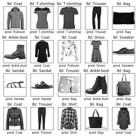
Let’s visualize the predictions on the test set
1
2
3
4
5
6
preds = model.predict_classes(x_test)

# plot 20 random data
rand_idxs = np.random.permutation(len(x_test))[:20]

plot(x_test[rand_idxs], y_test[rand_idxs], preds[rand_idxs])
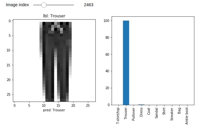
Interactive visualization
We can use Jupyter widgets to interactively visualize the results. Let’s plot the image, its acutal label and the predicted probabilities. Explaining Jupyter widgets is beyond the scope of this tutorial however, it is not very difficult to add interactivity to your notebooks. You can apply interact decorator to any function and make it interactive! For every function parameter, you have to define a widget that will act as an input and whenever, the widget’s state changes the decorated function will be called with new input values.
In the example below, we have a integer slider as the input widget. Whenever the slider is changed, the visualize_prediction function is called with the value of the slider assigned to the input parameter i.
1
2
3
4
5
6
7
8
9
10
11
12
13
14
from ipywidgets import interact, widgets
img_idx_slider = widgets.IntSlider(value=0, min=0, max=len(x_test)-1, description="Image index")

@interact(i=img_idx_slider)
def visualize_prediction(i=0):
    fix, (ax1, ax2) = plt.subplots(1, 2, figsize=(10, 5))
    ax1.imshow(x_test[i], cmap=plt.cm.binary)
    ax1.set_title(f"lbl: {class_names[y_test[i]]}")
    ax1.set_xlabel(f"pred: {class_names[preds[i]]}")


    ax2.bar(x=[class_names[i] for i in range(10)], height=probs[i]*100)
    plt.xticks(rotation=90)
You’ll get an output similar to the figure shown below. Change the slider and see it update instantly!
Conclusion
This post showed you how to train and test a simple feed forward neural network and visualize the data as well. In coming posts, we’ll improve the accuracy using convolutional neural networks.
This article is Part 2 in a 3-Part Tensorflow 2.0.


Comments