This article is Part 3 in a 5-Part Natural Language Processing with Python.
Introduction
Clustering is a process of grouping similar items together. Each group, also called as a cluster, contains items that are similar to each other. Clustering algorithms are unsupervised learning algorithms i.e. we do not need to have labelled datasets. There are many clustering algorithms for clustering including KMeans, DBSCAN, Spectral clustering, hierarchical clustering etc and they have their own advantages and disadvantages. The choice of the algorithm mainly depends on whether or not you already know how many clusters to create. Some algorithms such as KMeans need you to specify number of clusters to create whereas DBSCAN does not need you to specify. Another consideration is whether you need the trained model to able to predict cluster for unseen dataset. KMeans can be used to predict the clusters for new dataset whereas DBSCAN cannot be used for new dataset.
I’ve released a new hassle-free NLP library called jange. It is based on spacy and scikit-learn and provides very easy API for common NLP tasks. Here is a quick example to cluster documents.
1
2
3
4
5
6
7
8
9
10
11
12
13
14
15
16
17
18
19
20
from jange import ops, stream, vis
ds = stream.from_csv(
    "https://raw.githubusercontent.com/jangedoo/jange/master/dataset/bbc.csv",
    columns="news",
    context_column="type",
)
# Extract clusters
result_collector = {}
clusters_ds = ds.apply(
    ops.text.clean.pos_filter("NOUN", keep_matching_tokens=True),
    ops.text.encode.tfidf(max_features=5000, name="tfidf"),
    ops.cluster.minibatch_kmeans(n_clusters=5),
    result_collector=result_collector,
)
# Get features extracted by tfidf and reduce the dimensions
features_ds = result_collector[clusters_ds.applied_ops.find_by_name("tfidf")]
reduced_features = features_ds.apply(ops.dim.pca(n_dim=2))

# Visualization
vis.cluster.visualize(reduced_features, clusters_ds)
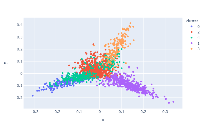
If you are interested then visit Github page to install and get started.
In this post we’ll cluster news articles into different categories. First download the dataset from http://mlg.ucd.ie/files/datasets/bbc-fulltext.zip and extract. The dataset consists of 2225 documents and 5 categories: business, entertainment, politics, sport, and tech. For most part, we’ll ignore the labels but we’ll use them while evaluating the trained model since many of the evaluation metrics need the “true” labels.
Let’s import the required libraries.
1
2
3
4
5
6
import pandas as pd
import numpy as np
from sklearn.cluster import MiniBatchKMeans
from sklearn.feature_extraction.text import TfidfVectorizer
from sklearn.decomposition import PCA
import matplotlib.pyplot as plt
Now we can read the data. If you look at the extracted zip, you’ll see there are 5 folders each containing articles. Each folder indicates a category and the articles contained in that folder belong to that category. As said before we aren’t concerned about the categories but it is there. To load data in this kind of format, sklearn has easy utility function called load_files which load text files with categories as subfolder names.
1
2
3
4
5
6
7
8
9
from sklearn.datasets import load_files

# for reproducibility
random_state = 0

DATA_DIR = "./bbc/"
data = load_files(DATA_DIR, encoding="utf-8", decode_error="replace", random_state=random_state)
df = pd.DataFrame(list(zip(data['data'], data['target'])), columns=['text', 'label'])
df.head()
| text | label | |
|---|---|---|
| 0 | Tate & Lyle boss bags top award\\n\\nTate & Lyle... | 0 |
| 1 | Halo 2 sells five million copies\\n\\nMicrosoft ... | 4 |
| 2 | MSPs hear renewed climate warning\\n\\nClimate c... | 2 |
| 3 | Pavey focuses on indoor success\\n\\nJo Pavey wi... | 3 |
| 4 | Tories reject rethink on axed MP\\n\\nSacked MP ... | 2 |
Feature extraction
For each article in our dataset, we’ll compute TF-IDF values. If you are not familiar with TF-IDF or feature extraction, you can read about them in the second part of this tutorial series called “Text Feature Extraction”.
1
2
3
vec = TfidfVectorizer(stop_words="english")
vec.fit(df.text.values)
features = vec.transform(df.text.values)
Now we have our feature matrix, we can feed to the model for training.
Model training
Let’s create an instance of KMeans. I’ll choose 5 as the number of clusters since the dataset contains articles that belong to one of 5 categories. Obviously, if you do not have labels then you won’t exactly know how many clusters to create so you have to find the best one that fits your needs via running multiple experiements and using domain knowledge to guide you.
Creating a model is pretty simple.
1
2
cls = MiniBatchKMeans(n_clusters=5, random_state=random_state)
cls.fit(features)
That is all it takes to create and train a clustering model. Now to predict the clusters, we can call predict function of the model. Note that not all clustering algorithms can predit on new datasets. In that case, you can get the cluster labels of the data that you used when calling the fit function using labels_ attribute of the model.
1
2
3
4
5
6
7
# predict cluster labels for new dataset
cls.predict(features)

# to get cluster labels for the dataset used while
# training the model (used for models that does not
# support prediction on new dataset).
cls.labels_
Visualization
To visualize, we’ll plot the features in a 2D space. As we know the dimension of features that we obtained from TfIdfVectorizer is quite large ( > 10,000), we need to reduce the dimension before we can plot. For this, we’ll ues PCA to transform our high dimensional features into 2 dimensions.
1
2
3
4
5
6
# reduce the features to 2D
pca = PCA(n_components=2, random_state=random_state)
reduced_features = pca.fit_transform(features.toarray())

# reduce the cluster centers to 2D
reduced_cluster_centers = pca.transform(cls.cluster_centers_)
Now that we have reduced our features and cluster centers into 2D, we can plot those points using a scatter plot. The first dimension will be used as X values and second dimension will be used as Y values in a XY plot. We also assign colors to each items using the predicted cluster labels so that items in a same cluster will be represented with same color. This is done by passing the labels to c parameter in scatter function. Again, if the clustering algorithm does not support predict function or if you want to visualize in the training data itself, you can also use c=cls.labels_ instead.
1
2
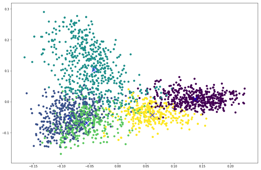
plt.scatter(reduced_features[:,0], reduced_features[:,1], c=cls.predict(features))
plt.scatter(reduced_cluster_centers[:, 0], reduced_cluster_centers[:,1], marker='x', s=150, c='b')
From the plot below we can see that apart from the rightmost cluster, others seems to be scattered all around and overlapping as well.
Evaluation
Evaluation for unsupervised learning algorithms is a bit difficult and requires human judgement but there are some metrics which you might use. There are two kinds of metrics you can use depending on whether or not you have the labels. For most of the clustering problems, you probably won’t have labels. If you had you’d do classification instead. But it is what it is. Here are a couple of them which I want to show you but you can read about other metrics on your own.
Evalauation with labelled dataset
If you have labelled dataset then you can use few metrics that give you an idea of how good your clustering model is. The one I’m going to show you here is homogeneity_score but you can find and read about many other metrics in sklearn.metrics module. As per the documentation, the score ranges between 0 and 1 where 1 stands for perfectly homogeneous labeling.
1
2
from sklearn.metrics import homogeneity_score
homogeneity_score(df.label, cls.predict(features))
1
0.7987538833468942
Evaluation with unlabelled dataset
If you don’t have labels for your dataset, then you can still evaluate your clustering model with some metrics. One of them is Silhouette Coefficient. From the sklearn’s documentation:
The Silhouette Coefficient is calculated using the mean intra-cluster distance (a) and the mean nearest-cluster distance (b) for each sample. The Silhouette Coefficient for a sample is (b - a) / max(a,b). To clarify, b is the distance between a sample and the nearest cluster that the sample is not a part of.
The best value is 1 and the worst value is -1. Values near 0 indicate overlapping clusters. Negative values generally indicate that a sample has been assigned to the wrong cluster, as a different cluster is more similar.
1
2
from sklearn.metrics import silhouette_score
silhouette_score(features, labels=cls.predict(features))
1
0.010641954485562228
So this value means that our clusters are overlapping. We can also see this in the plot above. Perhaps tuning different parameters for feature extractor and the clustering model will increase this score.
Conclusion
This post showed you how to cluster text using KMeans algorithm. You can cluster any kind of data, not just text and can be used for wide variety of problems. While the evaluation of clustering algorithms is not as easy compared to supervised learning models, it is still desirable to get an idea of how your model is performing. However, it is important to know what the metrics are measuring and if they are biased or have any limitations.
This article is Part 3 in a 5-Part Natural Language Processing with Python.


Comments