Multi output neural network in Keras (Age, gender and race classification)

Objective

• To learn how to create a model that produces multiple outputs in Keras
• To train a model that can predict age, gender and race of a person

Source code can be found at https://github.com/jangedoo/age-gender-race-prediction

Neural networks can produce more than one outputs at once. For example, if we want to predict age, gender, race of a person in an image, we could either train 3 separate models to predict each of those or train a single model that can produce all 3 predictions at once. In this short experiment, we’ll develop and train a deep CNN in Keras that can produce multiple outputs.

Dataset

We’ll use a dataset called UTKFace. UTKFace dataset is a large-scale face dataset with long age span (range from 0 to 116 years old). The dataset consists of over 20,000 face images with annotations of age, gender, and ethnicity.

The labels of each face image is embedded in the file name, formated like [age][gender][race]_[date&time].jpg

• [age] is an integer from 0 to 116, indicating the age
• [gender] is either 0 (male) or 1 (female)
• [race] is an integer from 0 to 4, denoting White, Black, Asian, Indian, and Others (like Hispanic, Latino, Middle Eastern).
• [date&time] is in the format of yyyymmddHHMMSSFFF, showing the date and time an image was collected to UTKFace.

Exploratory Analysis

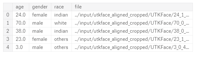
Let’s analyze our dataset. After parsing the filenames, I created a pandas dataframe with the following. Our input will be the image mentioned in the file column and the outputs will be rest of the colulmns.

Next, we’ll check the distribution of our dataset. First let’s group our dataset by gender and race and plot some charts.

fig, (ax1, ax2) = plt.subplots(1, 2, figsize=(15, 6))
_ = sns.boxplot(data=df, x='gender', y='age', ax=ax1)
_ = sns.boxplot(data=df, x='race', y='age', ax=ax2)

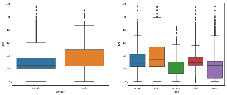
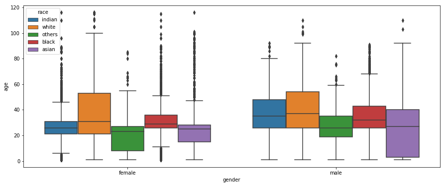
From the plot above, we can see that the most of the females are between 20 and 40 years old whereas males are between ~25 and ~50 years old. When grouped by race, we see that the age groups vary quite a lot. For even finer granularity, let’s plot a chart based on both gender and race.

plt.figure(figsize=(15, 6))
sns.boxplot(data=df, x='gender', y='age', hue='race')

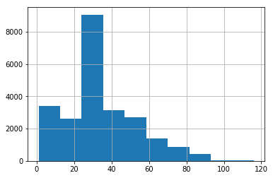
Since there is too much variation in distribution of data based on gender and rage. We’ll consider only a subset of data. After checking the histogram of age as shown below, we’ll only consider the data points that have age between 10 and 65.

Data Preparation

We’ll split our dataset into train, val and test. Training set consists of 70% of the data and test set consists remaining 30%. We’ll further split our training set again into 70/30 ratio for actual training set and validation set. Now the dataset contains 9079 images in training set, 3891 in validation set and 5559 in testing set.

Since our network produces multiple outputs, we’ll need to prepare our data accordingly. The following code returns a generator that produces the images and labels.

from keras.utils import to_categorical
from PIL import Image
 
def get_data_generator(df, indices, for_training, batch_size=16):
    images, ages, races, genders = [], [], [], []
    while True:
        for i in indices:
            r = df.iloc[i]
            file, age, race, gender = r['file'], r['age'], r['race_id'], r['gender_id']
            im = Image.open(file)
            im = im.resize((IM_WIDTH, IM_HEIGHT))
            im = np.array(im) / 255.0
            images.append(im)
            ages.append(age / max_age)
            races.append(to_categorical(race, len(RACE_ID_MAP)))
            genders.append(to_categorical(gender, 2))
            if len(images) >= batch_size:
                yield np.array(images), [np.array(ages), np.array(races), np.array(genders)]
                images, ages, races, genders = [], [], [], []
        if not for_training:
            break

For images, we read them, resize them and then normalize the pixel values between 0 and 1 by dividing them by 255. Next, for age, we’ll also divide it by max_age that we have in our dataset to normalize between 0 and 1. For races and genders, we convert them to one-hot encoded form. We don’t have to one-hot encode the gender since there are only two genders and a binary value can be used to represent it but we’ll use the categorical form.

Once we’ve accumulated enough samples, we yield X, y pair. Since there are multiple outputs, we put them in a list as shown below.

yield np.array(images), [np.array(ages), np.array(races), np.array(genders)]            

Make sure to remember the order of outputs. We’ll have to define our model accordingly.

Neural Network Model

The model is pretty straight forward CNN until the bottleneck layer as shown in the code below.

from keras.layers import Input, Dense, BatchNormalization, Conv2D, MaxPool2D, GlobalMaxPool2D, Dropout
from keras.optimizers import SGD
from keras.models import Model
 
def conv_block(inp, filters=32, bn=True, pool=True):
    _ = Conv2D(filters=filters, kernel_size=3, activation='relu')(inp)
    if bn:
        _ = BatchNormalization()(_)
    if pool:
        _ = MaxPool2D()(_)
    return _
 
input_layer = Input(shape=(IM_HEIGHT, IM_WIDTH, 3))
_ = conv_block(input_layer, filters=32, bn=False, pool=False)
_ = conv_block(_, filters=32*2)
_ = conv_block(_, filters=32*3)
_ = conv_block(_, filters=32*4)
_ = conv_block(_, filters=32*5)
_ = conv_block(_, filters=32*6)
bottleneck = GlobalMaxPool2D()(_)
 
# for age calculation
_ = Dense(units=128, activation='relu')(bottleneck)
age_output = Dense(units=1, activation='sigmoid', name='age_output')(_)
 
# for race prediction
_ = Dense(units=128, activation='relu')(bottleneck)
race_output = Dense(units=len(RACE_ID_MAP), activation='softmax', name='race_output')(_)
 
# for gender prediction
_ = Dense(units=128, activation='relu')(bottleneck)
gender_output = Dense(units=len(GENDER_ID_MAP), activation='softmax', name='gender_output')(_)
 
model = Model(inputs=input_layer, outputs=[age_output, race_output, gender_output])
model.compile(optimizer='rmsprop',
              loss={'age_output': 'mse', 'race_output': 'categorical_crossentropy', 'gender_output': 'categorical_crossentropy'},
              loss_weights={'age_output': 2., 'race_output': 1.5, 'gender_output': 1.},
              metrics={'age_output': 'mae', 'race_output': 'accuracy', 'gender_output': 'accuracy'})
# model.summary()

The bottleneck layer output 1D tensors. We’ll branch out from this layer into 3 separate paths to predict different labels. For predicting age, I’ve used bottleneck layer’s output as input to a dense layer and then feed that to another dense layer with sigmoid activation. Note that we’ve normalized our age between 0 and 1 so we have used sigmoid activation here. Similarly for race, I’ve used the same bottleneck output as input to another dense layer followed by the final dense softmax layer.

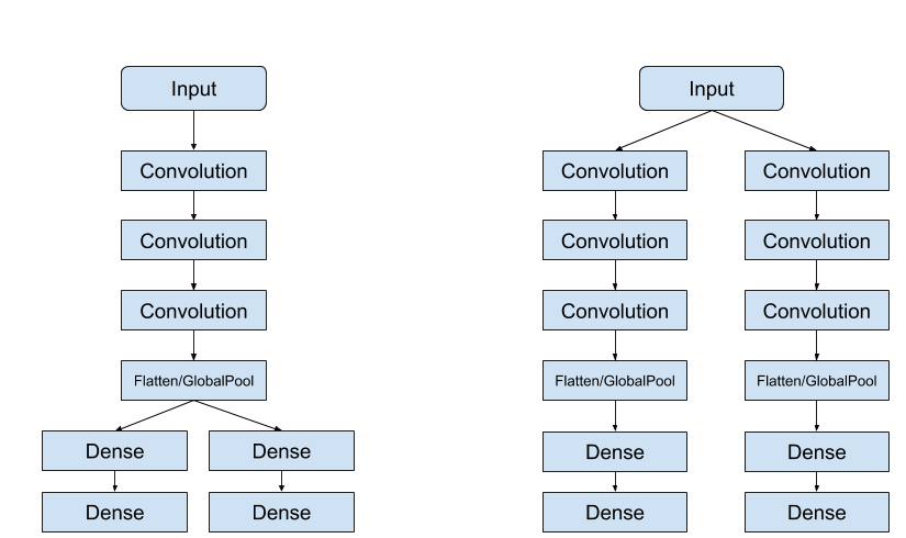
Our architecture is similar to the first diagram where we use the same convolution layers until we flatten and use separate dense layers for each of the outputs. In contrast, the right one branches off from the start. You can decide where to branch off and you can use as many layers as you want after branching off.

Another important part is that we need to specify different loss functions for different outputs. Age is a numeric value where as gender and race are categorical, so when we compile our model, we should specify which loss function we want to use. The loss of all outputs are combined together to produce a scalar value which is used for updating the network. The loss values may be different for different outputs and the largest loss will dominate the network update and will try to optimize the network for that particular output while discarding others. To overcome this, we can specify loss weights to indicate how much it will contribute towards the final loss. In this experiment, I’ve assigned 2 for age, 1.5 for race and 1 for gender. These values are hyper-parameters and you should try out different values depending on the task and dataset.

Training

I’ve trained the model for 10 epochs with batch size of 64. The plot below shows the model’s performance in training and validation set.

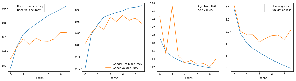
Our model is not performing well in the validation set. I suspect multiple reasons for this. First, we did not properly curate our dataset which was quite imbalanced. Also, the network seems to be overfitting, we could use dropout layers for regularization. We could also experiment with different optimizers and different loss weights.

Evaluation

Finally, let’s evaluate our model on test set and generate some predictions. It seems that our model is 87% accurate in predicting gender and 71% accurate in predicting the race. The classification report is only for 128 samples in test set but it shows that our model is pretty weak in classifying others race.

{'age_output_loss': 0.02968209301836269,
 'age_output_mean_absolute_error': 0.1393075646009556,
 'gender_output_acc': 0.8748183139534884,
 'gender_output_loss': 0.47691332462222075,
 'loss': 2.192765094513117,
 'race_output_acc': 0.717296511627907,
 'race_output_loss': 1.1043250560760498}
 
Classification report for race
             precision    recall  f1-score   support
 
          0       0.84      0.83      0.83        58
          1       0.69      0.93      0.79        29
          2       0.82      0.88      0.85        16
          3       0.70      0.44      0.54        16
          4       0.20      0.11      0.14         9
 
avg / total       0.74      0.76      0.74       128
 
 
Classification report for gender
             precision    recall  f1-score   support
 
          0       0.84      0.99      0.91        77
          1       0.97      0.73      0.83        51
 
avg / total       0.90      0.88      0.88       128

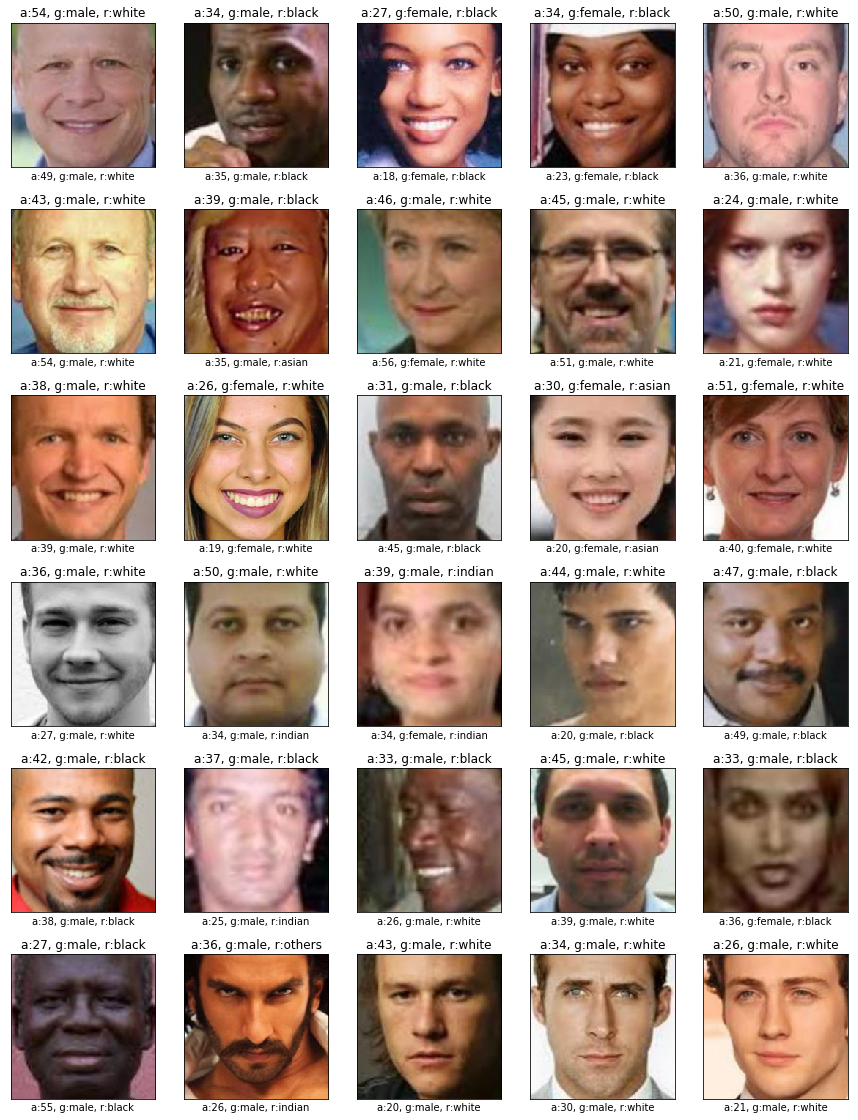
Figure below shows the predictions made by the model. Top label is predicted value and bottom label is actual value

To summarize, we trained a model that can produce multiple outputs and Keras makes it really easy to build such model.