Introduction
In Neural Networks, we use a non-linear activation function e.g. Sigmoid, TanH, ReLU etc. after layers like Linear/Dense or Conv2D etc. Consider a neural network with two hidden layers as shown below. The input is first passed through a Linear layer and then we apply an activation function ReLU which is then passed to the second hidden layer Linear2.
But why do we need to do so?
Neural Networks are used to learn data where the relationship between the inputs and outputs are non-linear. I’ll make this a bit more concrete in the sections below. We’ll train a couple of neural networks in Pytorch with and without non-linear activation function and visualize the differences. Hopefully that will give you some idea about the need of non-linearity in neural networks.
Data Setup
To be a bit more concrete, let’s consider a problem of classifying data points into one of two classes. We’ll use scikit-learn to generate a toy dataset. Before we dive into the process, lets import few libraries
Click to expand code
1
2
3
4
5
import torch
import numpy as np
from lets_plot import *
import pandas as pd
LetsPlot.setup_html()
Now, let’s generate a toy data set using make_moons function in scikit-learn and plot it.
1
2
3
4
5
from sklearn.datasets import make_moons
X, y = make_moons(n_samples=10000, noise=0.2, random_state=10)
df = pd.DataFrame(X, columns=['feature1', 'feature2'])
df['y'] = y
ggplot(df, aes('feature1', 'feature2', color='y')) + geom_point(size=0.7) + scale_color_discrete() + labs(title="Toy dataset")
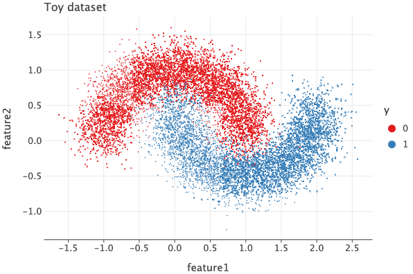
The data set we’ve generated have 2 input features and each data point belongs to one of two classes. I’ve chosen this dataset to highlight the importance of non-linearity.
If you were to take a single straight line and consider anything left to the line as ‘red’ and right to the line as ‘blue’, no matter how you place the line, there will always be points which will be mis-classified.
For e.g. if we were to draw a vertical line at 0.5 in x-axis, we’d classify a lot of blue points as red since there are many blue points to the left of this line and same with the red ones.
If we were to draw a horizontal line at -0.5 in y-axis, we’d classify all the red ones correctly, but also mis-classify a lot of blue ones as red.
There is simply no way a straight line can act as a proper decision boundary. This is to say that there is non-linear relationship between the inputs and outputs and hence we need to introduce non-linearity in our models.
Model
Now let’s create a couple of neural networks with and without non-linearity and see the differences between them. I’ll use Pytorch to create a simple neural network with two hidden layers.
Since our input has 2 features, the first layer takes (batch_size, 2) tensor as input and produces (batch_size, 10) tensor as output. We’ll use ReLU as a non-linear layer if enabled. The output from fc1 layer will be passed to ReLU. The output shape from ReLU is exactly same as its input i.e. (batch_size, 10).
Next, the fc2 layer produces an output of shape (batch_size, 2), where the first column indicates the logits (unnormalized scores) for class 0, and the second column indicates the logits for class 1. These logits can then be passed through a softmax function (during evaluation) to obtain class probabilities, or through argmax to determine the predicted class.
1
2
3
4
5
6
7
8
9
10
11
12
13
14
15
class DemoModel(torch.nn.Module):
    def __init__(self, use_relu=False):
        super().__init__()
        self.use_relu = use_relu
        self.fc1 = torch.nn.Linear(2, 10)
        self.fc2 = torch.nn.Linear(10, 2)

    def forward(self, x):
        x = self.fc1(x)
        if self.use_relu:
            x = torch.relu(x)
        return self.fc2(x)

linear_model = DemoModel(use_relu=False)
non_linear_model = DemoModel(use_relu=True)
Training
Below, I’ve defined a function called train which is a simple training loop. I’ve used torch.optim.AdamW optimizer and torch.nn.CrossEntropyLoss as loss function.
I’ve also created a train and test dataset and data loaders there.
Click to expand code
1
2
3
4
5
6
7
8
9
10
11
12
13
14
15
16
17
18
19
20
21
22
23
24
25
26
27
28
29
30
31
32
33
34
35
36
37
38
39
40
41
42
43
from sklearn.model_selection import train_test_split
from torch.utils.data import TensorDataset, DataLoader

def train(model: torch.nn.Module, train_dl, val_dl, epochs=10, ):
    optim = torch.optim.AdamW(model.parameters(), lr=1e-3)
    loss_fn = torch.nn.CrossEntropyLoss()
    losses = []
    for epoch in range(epochs):
        train_loss = 0.0
        model.train()
        for batch_X, batch_y in train_dl:
            optim.zero_grad()
            logits = model(batch_X)
            loss = loss_fn(logits, batch_y)
            loss.backward()
            optim.step()
            train_loss += loss.item() * batch_X.size(0)

        train_loss /= len(train_dl.dataset)

        model.eval()
        val_loss = 0.0
        with torch.no_grad():
            for batch_X, batch_y in val_dl:
                logits = model(batch_X)
                loss = loss_fn(logits, batch_y)
                val_loss += loss.item() * batch_X.size(0)

        val_loss /= len(val_dl.dataset)
        log_steps = int(0.2 * epochs)

        losses.append((train_loss, val_loss))
        if epoch % log_steps == 0 or epoch == epochs - 1:
            print(f'Epoch {epoch+1}/{epochs}, Training Loss: {train_loss:.4f}, Validation Loss: {val_loss:.4f}')

    return losses


X_train, X_test, y_train, y_test = train_test_split(torch.Tensor(X), torch.LongTensor(y))
train_ds = TensorDataset(X_train, y_train)
test_ds = TensorDataset(X_test, y_test)
train_dl = DataLoader(train_ds, shuffle=True, batch_size=32)
test_dl = DataLoader(test_ds, shuffle=False, batch_size=32)
Let’s train the two models for 50 epochs and see the train and validation loss curve.
1
2
linear_losses = train(linear_model, train_dl, test_dl, epochs=50)
non_linear_losses = train(non_linear_model, train_dl, test_dl, epochs=50)
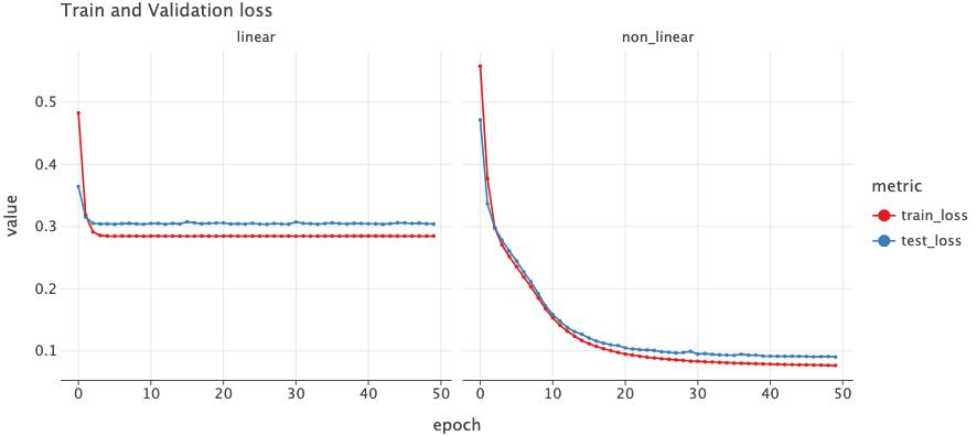
The plot on the left is for a model which does not use ReLU activation and the right one is for the model which does use ReLU activation. We can see a huge difference between the train/validation loss. The linear model’s loss does not decrease and stalls at around 0.29 where as the non_linear one sees decrease in loss throughout the epochs.
Evaluation
Let’s check the predictions of those two models. On the test set, the linear model has accuracy of 0.85 and the non-linear model has accuracy of 0.96 - a huge difference.
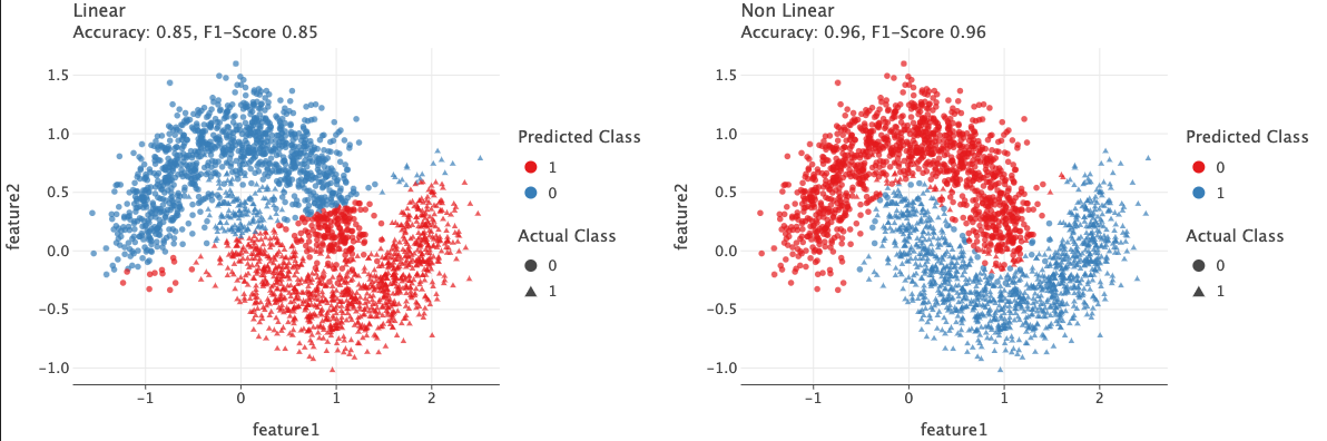
In the plot above, circles belong to class 0 and triangles belong to class 1.
We see the linear model has a sharp linear boundary where the points above this boundary are classified as 0 and below are classified as 1. Due to this, many points are mis-classified. In the left plot, ideally all circles should be in blue color and all triangles should be in red color, but this is not the case.
In the right plot, we see much better results. The model was able to learn a non-linear boundary that classifies 96% of the data points correctly.
Click to expand the code to generate above plot
1
2
3
4
5
6
7
8
9
10
11
12
13
14
15
16
17
from sklearn.metrics import classification_report
from lets_plot.mapping import as_discrete

def plot_classification(model, model_name: str):
    preds = model(X_test).argmax(dim=1).numpy()
    report_dict = (classification_report(y_test, preds, output_dict=True))
    plot_df = pd.DataFrame({"feature1": X_test[:, 0].numpy(), "feature2": X_test[: ,1].numpy(), "y": y_test, "pred": preds})
    title = f"{model_name}"
    subtitle = f"Accuracy: {report_dict['accuracy']:.2}, F1-Score {report_dict['weighted avg']['f1-score']:.2}"
    return ggplot(plot_df) + geom_point(aes('feature1', 'feature2', color=as_discrete('pred'), shape=as_discrete('y')), size=2.5, alpha=0.7) + labs(title=title, subtitle=subtitle, color="Predicted Class", shape="Actual Class")

fig_linear = plot_classification(linear_model, model_name="Linear")
fig_non_linear = plot_classification(non_linear_model, model_name="Non Linear")
bunch = GGBunch()
bunch.add_plot(fig_linear, 0, 0)
bunch.add_plot(fig_non_linear, 600, 0)
bunch
Activation visualization
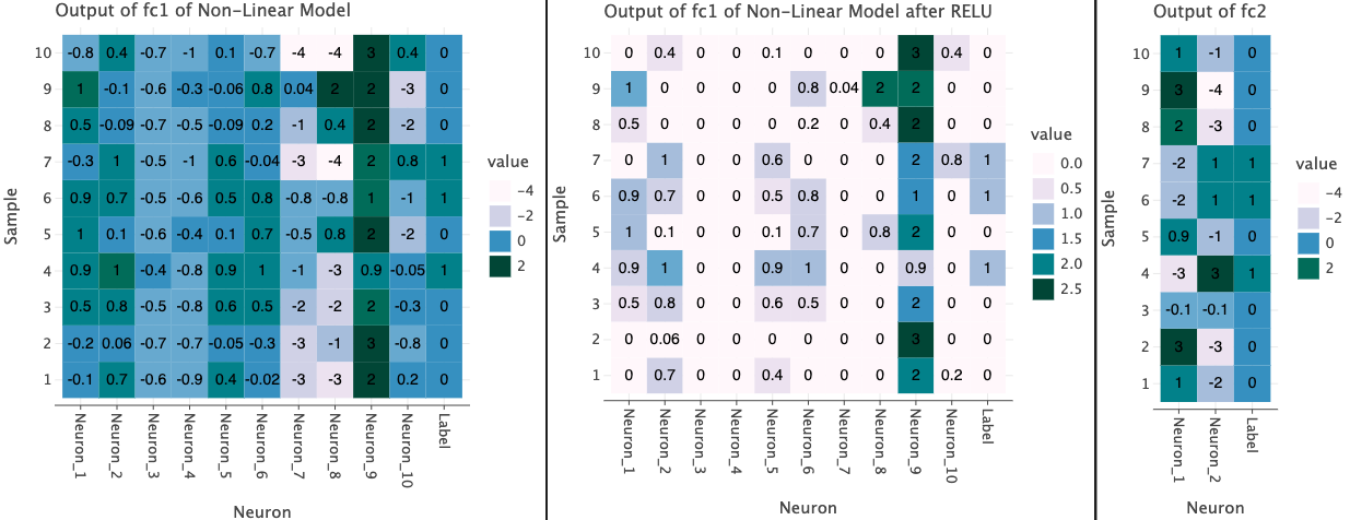
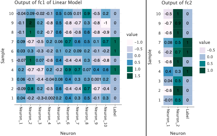
Now let’s look at the outputs from the individual layers in the model. I’ve taken first 10 rows from the test set and plotted the outputs from each layer below. I also show the true label of the each data point in the last column for reference.
In the plots below, I’ve used the both linear and non-linear model. Since the first layer takes produces a vector of size 10, we have 10 different values from each Neuron as well as a label column at the end for each sample.
The output of fc1 in both models contain a range of positive and negative values. This is obtained with a linear operation (matrix multiplication between input and layer’s weights).
However, when we use ReLU, we see that a non-linearity is introduced such that negative values are set to 0 and positive values are left unchanged. This means that only the positive values will contribute to the output of next layer.
Click to expand to generate code for plots above
1
2
3
4
5
6
7
8
9
10
11
12
13
14
15
16
17
18
19
20
21
22
23
24
25
26
27
28
29
30
31
32
33
34
35
36
37
38
39
40
41
42
43
44
45
46
47
48
49
50
def plot_activations(activations, labels, title: str):
    df_logits = pd.DataFrame(
        activations, columns=[f"Neuron_{i+1}" for i in range(activations.shape[1])]
    )
    df_logits['Label'] = labels
    df_logits["Sample"] = range(1, len(df_logits) + 1)


    df_logits = df_logits.melt(
        id_vars="Sample", var_name="Neuron"
    )
    return (
        ggplot(df_logits, aes("Neuron", as_discrete("Sample")))
        + geom_tile(aes(fill="value"))
        + geom_text(aes(label="value"), label_format=".1", color='black')
        + scale_fill_brewer(type='seq', palette=9)
        + labs(title=title)

    )

with torch.no_grad():
    logits_fc1 = non_linear_model.fc1(X_test[:10])
    logits_fc1_relu = torch.relu(logits_fc1)
    logits_fc2 = non_linear_model.fc2(logits_fc1_relu)

bunch = GGBunch()
bunch.add_plot(
    plot_activations(logits_fc1.numpy(), y_test[:10], title="Output of fc1 of Non-Linear Model"), 0, 0, 500, 500
)
bunch.add_plot(
    plot_activations(logits_fc1_relu.numpy(), y_test[:10], title="Output of fc1 of Non-Linear Model after RELU"), 502, -7, 500, 510
)
bunch.add_plot(
    plot_activations(logits_fc2.numpy(), y_test[:10], title="Output of fc2"), 872, 9, 500, 478
)

display(bunch)

bunch = GGBunch()
with torch.no_grad():
    linear_logits_fc1 = linear_model.fc1(X_test[:10])
    linear_logits_fc2 = linear_model.fc2(logits_fc1_relu)

bunch.add_plot(
    plot_activations(linear_logits_fc1.numpy(), y_test[:10], title="Output of fc1 of Linear Model"), 0, 0, 500, 500
)
bunch.add_plot(
    plot_activations(linear_logits_fc2.numpy(), y_test[:10], title="Output of fc2"), 375, 15, 500, 470
)
bunch
Conclusion
Although it is very well known to use non-linear activation functions in Neural Network, I hope I was able to give you a concrete visualization of why it is needed. Besides ReLU, there are many activation functions to choose e.g. SeLU, GeLU, Sigmoid, TanH etc. but ReLU seems to perform quite well despite very simple logic. Feel free to try out other activation functions and see what you get.
If you find any errors in this post, please let me know.


Comments