Introduction
Metric learning is an approach to train a model such that similar items have lower distance than dis-similar items in the vector space learned by the model. For example, if we have a photo of a dog as an input, the distance to another photo of a dog should be smaller compared to photos of other animals. In supervised classification problem, we aim to assign an item to a predefined set of classes but in metric learning, we aim to learn the representation that capture the underlying structure of the items. This is useful for applications which use similarity between items as the “main component” e.g. semantic search, clustering, recommender systems etc. You can read more about this topic in the paper A Tutorial on Distance Metric Learning.
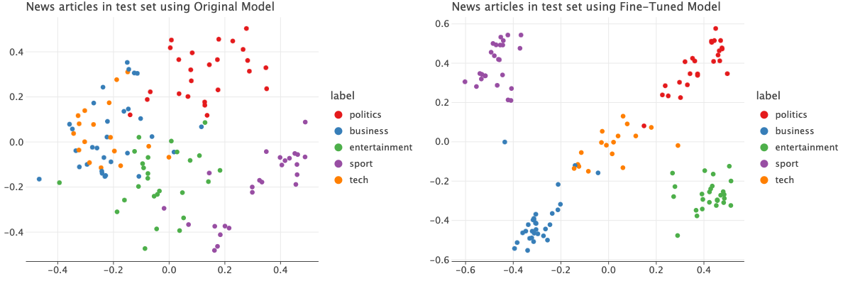
For example, consider the embeddings of news articles using a pre-trained model vs the one trained using the approach I’ll describe in this post. The difference is clear: the new embeddings are going to be more useful for tasks like custering compared to the old one.
When training a model, we use loss functions for metric learning such as Contrastive loss, Triplet loss etc. There are opensource libraries that already implement many of these. One of them is pytorch-metric-learning. For this post, I’ll focus on Triplet loss.
As the name indicates, triplet loss expects a list of triplets to compute the loss. Each triplet contains Anchor, Positive and Negative.
Anchor: This is the embedding of the item of concern. e.g. a photo of a dog
Positive: This is embedding of another item in the dataset which is similar to the Anchor
Negative: This is embedding of another item in the dataset which is not similar to the Anchor - in other words this item should be more dissimilar than the Positive
This loss function makes the model to minimize the distance between Anchor and Positive while maximizing the distance between Anchor and Negative. There are two concerns here: first is about the loss function itself. How do we write such a loss function? The second one is how do we create such dataset?
There are two ways to create such dataset. This process is also called ‘Triplet Mining’.
- Offline Triplet Mining: We create such dataset while pre-processing so that at the end we’ll have a huge list of triplets. Depending on the size of the original dataset, this list of triplets will be huge and need a lot of memory.
- Online Triplet Mining: Automatically generate these triplets using the data in a batch. This is the focus of this post.
All of this will be clear in the following sections.
Setup
Let me motivate this post with a toy example. Suppose we have a list of produce (fruits and vegetables) and we’d like the produce with same color to be closer to each other than the ones with different color. Maybe those embeddings will be used in a search engine where if a user submits a query “apple”, then we return fruits/vegetables which are red in color.
Before we dive in, I’ll import a few libraries and also load a small language model from SentenceTransformer. Note that I used Jupyter notebook to execute the code.
Click to expand code
1
2
3
4
5
6
7
8
import numpy as np
import torch
import pandas as pd
from lets_plot import *
LetsPlot.setup_html()

from sentence_transformers import SentenceTransformer
encoder = SentenceTransformer("all-MiniLM-L6-v2")
As mentioned above, let’s create a toy dataset where our “text” is the name of the produce and the label is the color.
1
2
3
4
5
6
7
8
9
10
11
12
13
14
id_to_label = dict(enumerate(["green", "red", "yellow"]))
label_to_id = {lbl:id for id, lbl in id_to_label.items()}
raw_data = [
    ("apple", "red"),
    ("banana", "yellow"),
    ("tomato", "red"),
    ("lemon", "yellow"),
    ("cucumber", "green"),
    ("spinach", "green"),
    ("pea", "green")
]

df = pd.DataFrame(raw_data, columns=["text", "label_str"])
df['label'] = df['label_str'].map(label_to_id)
Our goal is to have produce with same color to be near to each other in the vector space than the ones with different colors.
Triplet Mining
Let’s first focus on Online Triplet mining. Online Triplet Mining is an approach to generate Anchor, Positive, Negative triplets automatically from a batch of data. Typically the batch size is low e.g. 32, 64, 128 etc. so we can generate these triplets on-the-fly and compute the loss.
In this case, the Anchor is the items in our dataset. We have 7 produce in the dataset so there will be 7 Anchors. For each of those anchors, we find a positive and a negative item. To do that we first need the embeddings of the Anchors. Let’s use the encoder model we instantiated earlier to generate the embeddings.
1
2
3
embeddings = encoder.encode(df['text'].values, convert_to_tensor=True)
labels = torch.LongTensor(df['label'].values)
print(embeddings.shape, labels.shape) # torch.Size([7, 384]) torch.Size([7])
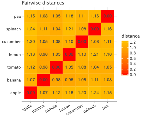
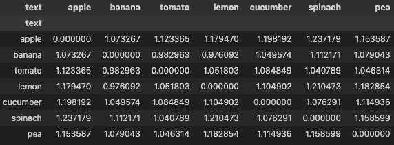
If we plot the pairwise distances between each pair, we see the following.
Click to expand code
1
2
3
4
5
6
7
8
9
10
11
distances = torch.cdist(embeddings, embeddings, p=2)
distances_df = pd.DataFrame(distances, columns=df['text'], index=df['text'])
melted_distances_df = distances_df.reset_index().melt(id_vars='text', var_name='text2', value_name='distance')
(
    ggplot(melted_distances_df, aes('text', 'text2', fill='distance'))
    + geom_tile()
    + scale_fill_gradient(high='orange', low='red')
    + geom_text(aes(label='distance'), label_format=".2f")
    + theme(axis_title_y=element_blank(), axis_title_x=element_blank())
    + labs(title="Pairwise distances")
)
Consider the row of ‘apple’. Since ‘tomato’ has red color, we want the distance between apple and tomato to be the least but this is not the case. That pair has a distance of 1.12 whereas apple and banana has the least distance of 1.07.
Since there are only two produce with color ‘red’, for Anchor=apple, we have positive=Tomato. Now for the negative, banana is the other item in our dataset which does not have the same label as apple i.e. color!=red and has the least distance. So banana will be the negative for apple. To summarize, we get the following triplet Anchor=apple, positive=tomato, negative=banana.
Let’s focus on ‘spinach’ which has color=green. To create a positive for this ‘spinach’, we look at the item with the same label which has the highest distance.
Distance of ‘spinach’ with ‘cucumber’ is 1.08, itself is 0 of course and 1.16 with ‘pea’. So we select ‘pea’ as its positive.
To create a negative, we look at item from different group which has the least distance. In this case, ‘tomato’ has the least distance (1.04). We finally have the following triplet Anchor=spinach, positive=pea, negative=tomato.
This positives and negatives we selected are also called HardPositives and HardNegatives since we selected the “extreme” items i.e. similar items with maximum distance and dis-similar items with minimum distance.
Do note that these triplets are generated for every batch, so as the model learns the selected positives and negatives for the same anchor will evolve over time.
Now let’s look at the triplets mined using this technique. I’ll use BatchHardMiner from pytorch-metric-learning library. We’ll implement our own but this will serve as a baseline to compare our implementation.
1
2
3
4
5
6
7
8
9
10
11
12
13
14
15
16
from pytorch_metric_learning.miners import BatchHardMiner
miner = BatchHardMiner()
anchors, positives, negatives = miner(embeddings, labels)
def get_mined_triplets_as_df(anchors, positives, negatives):
    return pd.DataFrame({
        "anchor": anchors,
        "positive": positives,
        "negative": negatives,
        "anchor_text": df.iloc[anchors]['text'].values,
        "positive_text": df.iloc[positives]['text'].values,
        "anchor_positive_dist": distances[anchors, positives],
        "negative_text": df.iloc[negatives]['text'].values,
        "anchor_negative_dist": distances[anchors, negatives]
    })

triplets_df = get_mined_triplets_as_df(anchors, positives, negatives)
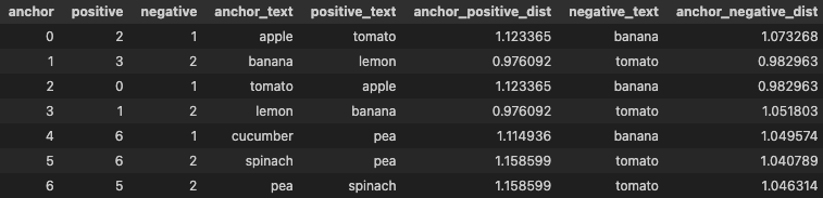
As we can see, for each item in our dataset, it generated positive and negative pair. I’ve also included the distance of the Anchor to Positive and Anchor to Negative as a reference.
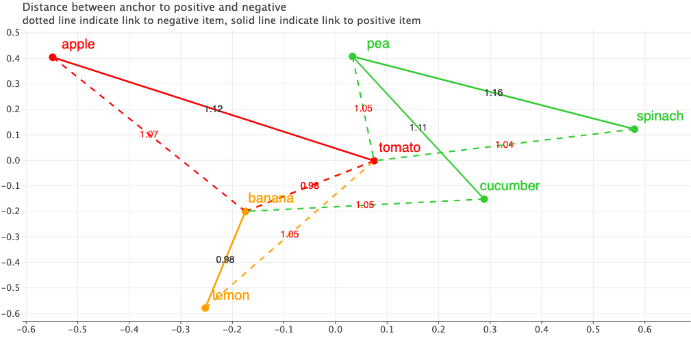
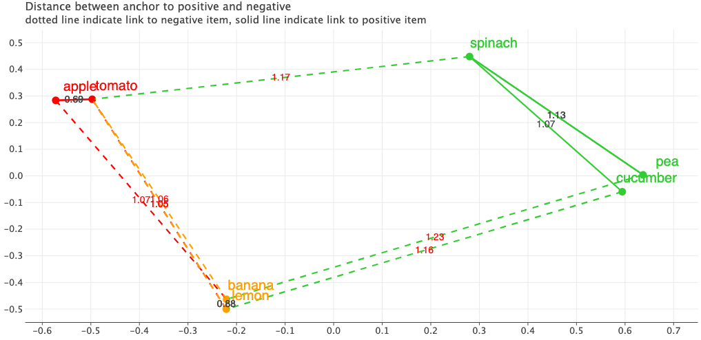
Let’s also visualize the triplets in their embedding space. The figure shows the Anchors in the 2D embedding space. I’ve applied PCA to reduce the dimensions to 2D. The solid lines indicate a link from Anchor to a Positive item and dotted line indicate a link from Anchor to Negative. The text on the line indicate the distance between each pair.
Looking at the current embeddings, the fruits are placed to the left side and vegetables to the right and seem to be closer to each other. But our goals are different. Produce with same color should be closer to each other.
Click to expand code
1
2
3
4
5
6
7
8
9
10
11
12
13
14
15
16
17
18
19
20
21
22
23
24
25
26
27
28
29
30
31
32
33
34
35
36
37
38
39
40
41
42
43
44
45
46
47
48
49
50
51
52
53
54
55
56
57
58
59
60
61
62
63
64
65
66
67
68
69
70
71
72
73
74
75
from sklearn.decomposition import PCA

def plot_triplets(embeddings: torch.Tensor, labels: torch.Tensor, df, miner):
    anchors, positives, negatives = miner(embeddings, labels)
    triplets_df = get_mined_triplets_as_df(anchors, positives, negatives)
    reduced_embeddings = PCA(n_components=2).fit_transform(embeddings)
    triplet_lines = []
    for idx, row in triplets_df.iterrows():
        triplet_lines.append({
            'x_start': reduced_embeddings[row['anchor'], 0],
            'y_start': reduced_embeddings[row['anchor'], 1],
            'x_end_pos': reduced_embeddings[row['positive'], 0],
            'y_end_pos': reduced_embeddings[row['positive'], 1],
            'x_end_neg': reduced_embeddings[row['negative'], 0],
            'y_end_neg': reduced_embeddings[row['negative'], 1],
            'dist_pos': row['anchor_positive_dist'],
            'dist_neg': row['anchor_negative_dist'],
            'anchor_label': id_to_label[labels[row['anchor']].item()]
        })

    plot_data = pd.DataFrame({
        'x': reduced_embeddings[:, 0],
        'y': reduced_embeddings[:, 1],
        'label': df['label_str'].values,
        'text': df['text'].values
    })
    triplet_lines_df = pd.DataFrame(triplet_lines)
    triplet_lines_df['x_mid_pos'] = (triplet_lines_df['x_start'] + triplet_lines_df['x_end_pos']) / 2
    triplet_lines_df['y_mid_pos'] = (triplet_lines_df['y_start'] + triplet_lines_df['y_end_pos']) / 2

    triplet_lines_df['x_mid_neg'] = (triplet_lines_df['x_start'] + triplet_lines_df['x_end_neg']) / 2
    triplet_lines_df['y_mid_neg'] = (triplet_lines_df['y_start'] + triplet_lines_df['y_end_neg']) / 2

    plot = (
        ggplot() +
        geom_point(aes('x', 'y', color='label'), data=plot_data, size=5, show_legend=False)

        # Arrows to positive samples
        + geom_segment(
            aes(x='x_start', y='y_start', xend='x_end_pos', yend='y_end_pos',
                color='anchor_label', label='dist_pos'),
            data=triplet_lines_df,
            arrow=arrow(type='closed', angle=15, length=0.1),
            size=1,
            show_legend=False
        )

        # # Arrows to negative samples
        + geom_segment(
            aes(x='x_start', y='y_start', xend='x_end_neg', yend='y_end_neg',
                color='anchor_label', label='dist_neg'),
            data=triplet_lines_df,
            arrow=arrow(type='closed', angle=15, length=0.1),
            size=1,
            linetype='dashed',
            show_legend=False
        )

        + geom_text(aes(x='x_mid_pos', y='y_mid_pos', label='dist_pos'),
                data=triplet_lines_df, size=7, va='center', label_format=".2f")

        + geom_text(aes(x='x_mid_neg', y='y_mid_neg', label='dist_neg'),
                data=triplet_lines_df, size=7, va='center', color='red', label_format=".2f")

        + geom_text(aes('x', 'y', label='text', color='label'), data=plot_data, size=10, nudge_x=0.05, nudge_y=0.05, show_legend=False)

        + scale_color_manual(values={'red': 'red', 'green': '#32CD32', 'yellow': '#FFA000'})

        + ggsize(1024, 500)
        + theme(axis_title=element_blank())
        + labs(title="Distance between anchor to positive and negative", subtitle="dotted line indicate link to negative item, solid line indicate link to positive item")
    )
    return plot

plot_triplets(embeddings=embeddings, labels=labels, df=df, miner=miner)
Ok, so far we’ve seen how Online Triplet Mining works and how to use an existing implementation. Now let’s implement our own version.
To start, we have embeddings of each item in a batch and their labels. Once again, the shape of embeddings is (batch_size, embed_dim) and shape of labels is (batch_size,) i.e. a 1D tensor.
Since we need to calculate the distance between each pair in the batch, first we compute the distance. Using torch.cdist with p=2 will calculate Euclidean distance.
1
2
distances = torch.cdist(embeddings, embeddings, p=2)
display(pd.DataFrame(distances, columns=df['text'], index=df['text']))
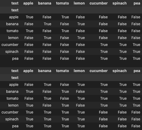
Next, we create masks. For each entry in the distances matrix, we’ll create a positive mask whose True value indicates that the distance is for positive pair. Same for negative mask, whose True value indicates that the distance is for negative pair.
Since labels is a 1D array and we need a 2D mask, we do a little bit of broadcasting magic.
1
2
3
4
5
6
7
labels2 = labels.unsqueeze(1) # (N, 1)
positive_mask = labels2 == labels2.t() # (N, N) bool tensor (True indicates the pair is positive)

negative_mask = labels2 != labels2.t() # (N, N) bool tensor (True indicates the pair is negative)

display(pd.DataFrame(positive_mask, columns=df['text'], index=df['text']))
display(pd.DataFrame(negative_mask, columns=df['text'], index=df['text']))
The figure below shows how the positive_mask and negative_mask look like.
Now let’s see how these masks are used to find positives and negatives.
1
2
3
4
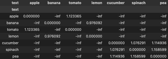
distances_masked = distances.masked_fill(negative_mask, float('-inf'))
display(pd.DataFrame(distances_masked, columns=df['text'], index=df['text']))
# for positive pairs, we want the item with least similarity i.e. max distance from same group
_, hard_positive_ids = torch.max(distances_masked, dim=-1)
As seen in the figure below, to find the positives, we set the values to -inf for entries which belong to different class or group. Now for each anchor, we find the item with highest distance.
 Now the
 hard_positive_ids has the following tensor([2, 3, 0, 1, 6, 6, 5])
Similarly to find the negatives, we replace the distance of items from same group with inf. The remaining “valid distances” are only for items from different group. Then for each anchor we find the item with smallest distance.
1
2
3
4
distances_masked = distances.masked_fill(positive_mask, float('inf'))
display(pd.DataFrame(distances_masked, columns=df['text'], index=df['text']))
# for each anchor, find the item with lowest distance which does not belong to same group
_, hard_negative_ids = torch.min(distances_masked, dim=-1)
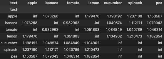 Now
Now hard_negative_ids contains the following tensor([1, 2, 1, 2, 1, 2, 2])
Let’s package this in a class so that we can use it easily later.
1
2
3
4
5
6
7
8
9
10
11
12
13
14
15
16
17
18
19
20
21
22
23
24
25
class MyMiner:
    def __call__(self, embeddings: torch.Tensor, labels: torch.Tensor):
        n_items = embeddings.size(0)
        anchors = torch.arange(n_items)

        distances = torch.cdist(embeddings, embeddings, p=2)

        labels = labels.unsqueeze(1) # (N, 1)
        positive_mask = labels == labels.t() # (N, N) bool tensor (True indicates the pair is positive)
        negative_mask = labels != labels.t() # (N, N) bool tensor (True indicates the pair is negative)


        # fill the distances of negative pairs with negative infinity value
        # the remaining distances are for positive pairs only, and we find the positive
        # item with highest distance as hard positive
        _, positives = torch.max(distances.masked_fill(negative_mask, float('-inf')), dim=1)
        # fill the distances of positive pairs with positive infinity value
        # the remaining distances are for negative pairs only, and we find the negative item
        # with lowest distance as hard negative
        _, negatives = torch.min(distances.masked_fill(positive_mask, float('inf')), dim=1)

        return anchors, positives, negatives

myminer = MyMiner()
plot_triplets(embeddings=embeddings, labels=labels, df=df, miner=myminer)
If we plot the triplets, we get exactly the same results as before when we used an open source implementation.

Triplet Loss
Triplet loss is quite straightforward. The formula is
\[loss = max(dist_{ap} - dist_{an} + margin, 0)\]where
\(dist_{ap}\) = Distance between Anchor and Positive
\(dist_{an}\) = Distance between Anchor and Negative
We compute the loss for each triplet and typically take the mean as final loss value.
The following code walks through each step.
1
2
3
4
5
6
7
8
9
10
11
12
# we want the distance between anchor/positive to be at least 'margin' amount greater than anchor/negative
# value of margin depends on the distance function used. here we are using Euclidean distance
margin = 0.05
# compute difference between positive and negative item's distance
triplets_df['diff_ap_an'] = triplets_df['anchor_positive_dist'] - triplets_df['anchor_negative_dist']
# add margin
triplets_df['diff_ap_an_plus_marin'] = triplets_df['diff_ap_an'] + margin
# clip negative values to zero
triplets_df['clipped'] = np.clip(triplets_df['diff_ap_an_plus_marin'], a_min=0, a_max=None)
display(triplets_df)
loss = triplets_df['clipped'].mean()
print(f"Triplet margin loss = {loss:5f}")
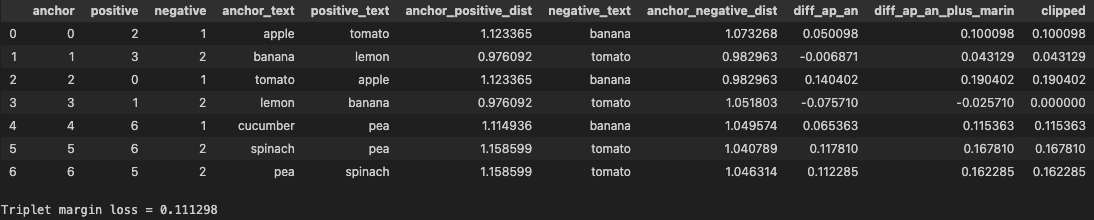
The calculation should be straight forward. The clipped column contains the loss for each triplet and the at the end we take average as final loss for the batch.
Let’s focus on the case where the anchor is lemon to understand about the role of margin. The triplet is Anchor=lemon, positive=banana(dist. 0.97), negative=tomato(dist 1.05). The loss for this triplet is 0. Why?
The positive item for lemon already has distance less than the negative item. The difference is -0.0757 which is lower than our margin of 0.05. Even after we add the margin we get -0.0257 which gets clipped to 0. This means the model already does what it is supposed to do in this case i.e. bring positive closer to the anchor compared to the negative.
Same for the case when banana is anchor. The positive item has less distance than negative one. The difference is -0.0068 and after adding the margin we get 0.0431 as the loss which is low compared to loss values for other triplets.
Now that we know how to calculate Triplet Loss, let’s implement a proper version and compare it against Pytorch and pytorch-metric-learning’s implementation.
1
2
3
4
5
6
7
8
9
10
11
12
13
14
15
16
17
18
19
20
21
22
23
24
25
26
27
28
29
30
31
32
33
34
35
36
37
38
39
40
41
42
class TripletLoss:
    def __init__(self, margin=0.05, p=2):
        self.margin = margin
        self.p = p

    def __call__(self, anchors, positives, negatives):
        ap = torch.pairwise_distance(anchors, positives, p=self.p)
        an = torch.pairwise_distance(anchors, negatives, p=self.p)

        # the above step is basically same as the following

        # anchors = torch.nn.functional.normalize(anchors, p=self.p, dim=-1)
        # positives = torch.nn.functional.normalize(positives, p=self.p, dim=-1)
        # negatives = torch.nn.functional.normalize(negatives, p=self.p, dim=-1)
        # ap = (anchors - positives).pow(2).sum(dim=-1).sqrt()
        # an = (anchors - negatives).pow(2).sum(dim=-1).sqrt()

        # we can use relu since it keep positive values as is and assigns negative values to 0
        # return torch.relu(ap - an + self.margin).mean()
        # pytorch uses the version shown below
        # https://pytorch.org/docs/main/_modules/torch/nn/functional.html#triplet_margin_loss
        return torch.clamp_min(self.margin + ap - an, 0).mean()

from pytorch_metric_learning.losses import TripletMarginLoss
from pytorch_metric_learning.reducers import MeanReducer

anchor_ids, positive_ids, negative_ids = myminer(embeddings=embeddings, labels=labels)
anchors = embeddings[anchor_ids]
positives = embeddings[positive_ids]
negatives = embeddings[negative_ids]
# pytorch implementation
torch_loss = torch.nn.TripletMarginLoss(margin=0.05, p=2, swap=False)(
    anchors, positives, negatives
)
# pytorch metric learning implementation. by default uses Euclidean distance
# we also specify MeanReducer to take average of individual triplet loss
pml_loss = TripletMarginLoss(
    margin=0.05, swap=False, smooth_loss=False, reducer=MeanReducer()
)(embeddings, labels, (anchor_ids, positive_ids, negative_ids))
# our implementation
my_loss = TripletLoss(margin=0.05, p=2)(anchors, positives, negatives)
print(f"Torch loss: {torch_loss:7f}. PML loss: {pml_loss:7f}. My loss: {my_loss:.7f}")
1
Torch loss: 0.111298. PML loss: 0.111298. My loss: 0.1112983
So, all 3 implementations give the same output. We know our implementation works!
Usage
Now let’s use the miner and the loss function we just implemented. We’ll finetune the base model i.e. the SentenceTransformer model we instantiated earlier for our toy example.
Below is our model. In the training_step method you can see how we use the miner and the loss function.
1
2
3
4
5
6
7
8
9
10
11
12
13
14
15
16
17
18
19
20
21
22
23
24
25
26
27
28
29
30
31
32
import pytorch_lightning as L
import copy
class MyModel(L.LightningModule):
    def __init__(self, encoder):
        super().__init__()
        # copy the original model so that we have a fresh copy
        self.encoder = copy.deepcopy(encoder)

    def forward(self, input_ids: torch.Tensor, attention_mask: torch.Tensor, **kwargs):
        # sentence transformer model expects a dict as input
        outputs = self.encoder(dict(input_ids=input_ids, attention_mask=attention_mask, **kwargs))
        # sentence transformer model returns pooled token embeddings as 'sentence_embedding'
        embeddings = outputs['sentence_embedding']
        return embeddings

    def training_step(self, batch, batch_idx):
        miner = MyMiner()
        labels = batch.pop('labels')
        embeddings = self(**batch)

        anchor_ids, positive_ids, negative_ids = miner(embeddings, labels)
        anchors = embeddings[anchor_ids]
        positives = embeddings[positive_ids]
        negatives = embeddings[negative_ids]
        loss = TripletLoss(margin=0.05, p=2)(anchors, positives, negatives)
        self.log('train_loss', loss, on_epoch=True, on_step=True, prog_bar=True)
        return loss

    def configure_optimizers(self):
        return torch.optim.AdamW(self.parameters(), lr=4e-5)

model = MyModel(encoder=encoder)
Toy Dataset
Now I’ll commit a crime by training on our small dataset of 7 items and then evaluating on the same dataset but this is just to show that things are working end-to-end. After this section, we’ll use this in a proper dataset with proper train test split.
The code to generate the DataLoader and train the model is hidden. You can check it out if you want to follow along.
Click to expand code
1
2
3
4
5
6
7
8
9
10
11
12
13
14
15
16
17
18
19
20
21
22
23
24
25
26
27
28
29
30
31
import datasets
from torch.utils.data import DataLoader
ds = datasets.Dataset.from_pandas(df)
def tokenize(batch):
    return encoder.tokenize(batch['text'])
ds = ds.map(tokenize, batched=True)

from transformers import DataCollatorWithPadding
columns = ['input_ids', 'attention_mask', 'token_type_ids', 'label']

# we'll not use this test set anyways while training, you might want to change it
ds_dict = ds.train_test_split(test_size=0.01)

train_ds = ds_dict['train']
test_ds = ds_dict['test']

train_dl = DataLoader(
    train_ds.select_columns(columns),
    shuffle=True,
    batch_size=64,
    collate_fn=DataCollatorWithPadding(tokenizer=encoder.tokenizer),
)
test_dl = DataLoader(
    test_ds.select_columns(columns),
    shuffle=False,
    batch_size=32,
    collate_fn=DataCollatorWithPadding(tokenizer=encoder.tokenizer),
)

trainer = L.Trainer(fast_dev_run=False, max_epochs=5)
trainer.fit(model, train_dataloaders=train_dl, val_dataloaders=test_dl)
I trained it for 5 epochs and now if we plot the pairwise distances again, we see the following.
 Now as we expected, apple and tomato have the least distance compared to all other pairs. All the green vegetable pairs have less distance compared to other pairs. Lemon and Banana are also closer than ever.
Just for fun, let’s visualize how different the mined triplets would look like using the embeddings from the fine-tuned model.
1
2
3
# use the new encoder to generate embeddings
embeddings = model.encoder.encode(df['text'], convert_to_tensor=True)
plot_triplets(embeddings=embeddings, labels=labels, df=df, miner=miner)
Did you see the difference? Before, all fruits were roughly on the left side and vegetables were on the right side and were quite far apart. But now our produce are clustered together based on the color i.e. the objective we defined and trained on!
News Dataset
Let’s see our implement in action in a relatively big dataset compared to our toy dataset. I’ll use the dataset from HuggingFace hub which contains news articles. Our goal is to make sure the embeddings of news articles from same category are similar than the ones from other category. The embeddings generated will be especially useful for semantic search and clustering.
1
2
news_ds = datasets.load_dataset("SetFit/bbc-news", split="train") # fields: ['text', 'label', 'label_text']
news_model = MyModel(encoder=encoder)
Click to expand training code
1
2
3
4
5
6
7
8
9
10
11
12
13
14
15
16
17
18
19
20
21
22
23
24
25
def tokenize(batch):
    return encoder.tokenize(batch['text'])
news_ds = news_ds.map(tokenize, batched=True)
columns = ['input_ids', 'attention_mask', 'token_type_ids', 'label']

ds_dict = news_ds.train_test_split(test_size=0.1)

train_ds = ds_dict['train']
test_ds = ds_dict['test']

train_dl = DataLoader(
    train_ds.select_columns(columns),
    shuffle=True,
    batch_size=64,
    collate_fn=DataCollatorWithPadding(tokenizer=encoder.tokenizer),
)
test_dl = DataLoader(
    test_ds.select_columns(columns),
    shuffle=False,
    batch_size=32,
    collate_fn=DataCollatorWithPadding(tokenizer=encoder.tokenizer),
)

trainer = L.Trainer(fast_dev_run=False, max_epochs=5)
trainer.fit(news_model, train_dataloaders=train_dl, val_dataloaders=test_dl)
I trained it for 5 epochs. Now let’s plot the embeddings using the original model and the fine tuned model.
1
2
original_embeddings = encoder.encode(test_ds['text'])
new_embeddings = news_model.encoder.encode(test_ds['text'])
The difference between the embeddings from the pre-traine and the fine-tuned model is drastic. The new embeddings are quite well separated according to the labels compared to the old one.
Click to expand visualization code
1
2
3
4
5
6
7
8
9
10
11
12
13
14
15
16
17
18
19
20
21
22
23
24
25
26
27
28
29
def plot_embeddings(embeddings, labels, title):
    reduced_embeddings = PCA(n_components=2).fit_transform(embeddings)
    df = pd.DataFrame({
        "x": reduced_embeddings[:, 0],
        "y": reduced_embeddings[: ,1],
        "label": labels
    })
    fig = (
        ggplot(df, aes('x', 'y', color='label'))
        + geom_point()
        + labs(title=title)
        + theme(axis_title=element_blank())
    )
    return fig

fig1 = plot_embeddings(
    original_embeddings,
    test_ds["label_text"],
    title="News articles in test set using Original Model",
)
fig2 = plot_embeddings(
    new_embeddings,
    test_ds["label_text"],
    title="News articles in test set using Fine-Tuned Model",
)
bunch = GGBunch()
bunch.add_plot(fig1, 0, 0, 600, 400)
bunch.add_plot(fig2, 600, 0, 600, 400)
display(bunch)
Benchmarking
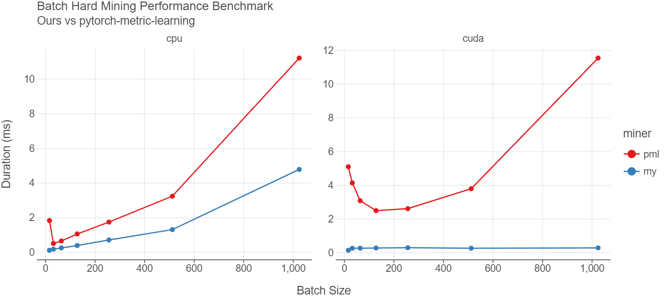
To compare the runtime performance of our implementation of miner vs the one in pytorch-metric-learning, I’ve created a small benchmark.
One of the main highlights of our implementation is that everything is done via tensor operations. There is no for loop. This is critical because when training, the embeddings will be in GPU. Now if we were to copy the embeddings to CPU and then run the operations, it would be slow because copying from GPU to CPU takes time and GPU is much faster for vectorized operations than CPU. Besides, after finding the triplets in CPU, we’d again have to copy those triplets to GPU adding more latency. For example, in Open Metric Learning’s HardTripletMiner code, they use for-loops which will make things slower.
Click to expand benchmark code
1
2
3
4
5
6
7
8
9
10
11
12
13
14
15
16
17
18
19
20
21
22
23
24
25
26
27
28
29
30
31
32
33
34
35
36
37
38
39
40
41
42
43
44
45
46
47
48
49
50
51
52
53
54
55
56
57
58
59
60
61
62
63
64
65
66
67
68
69
70
71
72
73
74
75
76
77
78
79
80
# load a model to generate embeddings
from sentence_transformers import SentenceTransformer
encoder = SentenceTransformer("all-MiniLM-L6-v2")

# load a dataset
import datasets
news_ds = datasets.load_dataset("SetFit/bbc-news", split="train")

# extract embeddings and make this available in cpu
embeddings = encoder.encode(news_ds['text'], convert_to_tensor=True).cpu()
labels = torch.LongTensor(news_ds['label'])

# copy embeddings and labels to GPU
cuda_embeddings = embeddings.cuda()
cuda_labels = labels.cuda()

# instantiate miners
from pytorch_metric_learning.miners import BatchHardMiner

pml_miner = BatchHardMiner()
my_miner = MyMiner()

# before moving forward let's make sure we have same output from both miners
pml_anchors, pml_positives, pml_negatives = pml_miner(embeddings, labels)
my_anchors, my_positives, my_negatives = my_miner(embeddings, labels)
assert torch.equal(pml_anchors, my_anchors)
assert torch.equal(pml_positives, my_positives)
assert torch.equal(pml_negatives, my_negatives)

# benchmark function
import time
def benchmark(embeddings, labels, miner, n_runs=10):
    """returns avg and std of time to mine in milliseconds"""
    durations = []
    for _ in range(n_runs):
        start = time.monotonic()
        _ = miner(embeddings, labels)
        end = time.monotonic()
        durations.append((end - start) * 1000)
    return np.mean(durations), np.std(durations)

batch_sizes = [16, 32, 64, 128, 256, 512, 1024]
miners = [('pml', pml_miner), ('my', my_miner)]

rows = []
for batch_size in batch_sizes:
    batch_embeddings = embeddings[:batch_size]
    batch_labels = labels[:batch_size]

    batch_cuda_embeddings = cuda_embeddings[:batch_size]
    batch_cuda_labels = cuda_labels[:batch_size]

    for miner_name, miner in miners:
        mean, std = benchmark(batch_embeddings, batch_labels, miner, n_runs=20)
        rows.append({
            "bs": batch_size,
            "miner": miner_name,
            "duration_ms": mean,
            "duration_std" : std,
            "device": "cpu"
        })

        mean, std = benchmark(batch_cuda_embeddings, batch_cuda_labels, miner, n_runs=20)
        rows.append({
            "bs": batch_size,
            "miner": miner_name,
            "duration_ms": mean,
            "duration_std" : std,
            "device": "cuda"
        })

stats_df = pd.DataFrame(rows)
fig = (
    ggplot(stats_df, aes('bs', 'duration_ms', color='miner'))
    + geom_line()
    + geom_point()
    + facet_wrap('device', nrow=1, scales='free')
    + labs(title="Batch Hard Mining Performance Benchmark", subtitle="Ours vs pytorch-metric-learning", y="Duration (ms)", x="Batch Size")
)
display(fig)
As seen from the figure above, our implementation is much faster than the one in pytorch-metric-learning library. In CPU, our implementation is about 3 times faster for almost all batch sizes. The difference is even more visible when the embeddings and labels are in GPU. For almost all the batch sizes, our implementation takes about 0.3 milliseconds whereas the pml implementation takes more time as the batch size increases. When batch size is 1024, pml takes about 11.55 ms vs 0.28 ms giving us 41x improvement in runtime performance.
I didn’t benchmark the miner from “Open Metric Learning” but since it uses for loop, I am very sure it will be pretty slow compared to ours or pml. Having said that since model training time typically takes hours, if not days, small sub-second differences should not be a big issue. Just choose a library that suits your needs.
Conclusion
In this post explored one of many ways to generate positive and negative pairs on the fly. There are two libraries which provide many other approaches to mine as well as loss functions. One is called pytorch-metric-learning and another is Open Metric Learning. You can check those libraries for more details.
I hope this post was useful. Please let me know if you found any errors.


Comments