Multi-Head Attention From Scratch

This article is Part 1 in a 5-Part Understanding Transformers Architecture.

• Part 1 - > Multi-Head Attention From Scratch
• Part 2 - Masking in Transformer Encoder/Decoder Models
• Part 3 - Implementing Transformer Encoder Layer From Scratch
• Part 4 - Implementing Transformer Decoder Layer From Scratch
• Part 5 - Decoding strategies in Decoder models (LLMs)

Introduction

In this post, we’ll implement Multi-Head Attention layer from scratch using Pytorch. We’ll also compare our implementation against Pytorch’s implementation and use this layer in a text classification task. Specifically we’ll do the following:

• Implement Scaled Dot Product Attention
• Implement our own Multi-Head Attention (MHA) Layer
• Implement an efficient version of Multi-Head Attention Layer
• Use our two implementations and Pytorch’s implementation in a model to classify texts and evaluate their performance
• Implement Positional Embeddings and see why they are useful

I’ve tried to explain each step in detail as much as possible so some of the details may be obvious to many but I will cover them here anyways. Overall idea of MHA is pretty straightforward but when implementing it I faced many issues especially related to reshaping of the tensors. So this post is also for my own sake because I want to refer to these implementation details for reference as well.

Ok, now let’s begin. Since you are already here I guess you know Multi-Head Attention layer is the backbone for Transformer architecture. Many recent models including ChatGPT, Gemini, LLama etc. are based on Transformer architecture. This was introduced in a paper called Attention Is All You Need. As mentioned above, in this post we’ll just focus on Multi-Head Attention layer.

Scaled Dot Product Attention

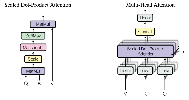
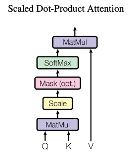
Let’s focus on one of many approaches to calculate attention - Scaled Dot Product Attention. The figure below (taken from the paper shared above) shows how scaled dot product attention is calculated.

Let’s look at the formula first.

\[Attention(Q,K,V) = (Attention\_Weights ) V\]

where, \(Attention\_Weights = softmax(\frac{QK^T}{\sqrt{d_k}})\)

This function \(Attention\) accepts 3 matrices: Query, Key and Value. What are those?

For the sake of this discussion, I’ll NOT consider batched operation so there is no batch dimension. During implemetation we’ll take care of it. Let’s say we have a single text (i.e. sequence) how are you. When using a tokenizer, we’ll get something like

Token	Token ID
how	10
are	3
you	5

Once we pass the token ids through an embedding layer, we’ll obtain a vector for each token. Let’s say our embedding dimension is 2, so the embeddings matrix for this sequence will have a shape of \(3 \times 2\)

\[\begin{bmatrix} 1.1 & 1.2\\ 2.1 & 2.2\\ 3.1 & 3.2 \end{bmatrix}_{3\times2}\]

Typically this kind of embedding matrix is used as Query, Key and Value in the first Multi-Head Attention Layer. Output of previous layers are also used as long as they are in the required shape i.e. (sequence_length, embedding_dim). To limit the scope of this post, I’ll focus on a variant called self-attention where same embedding matrix is passed as Query, Key and Value.

Intuition

Let’s look at the formula to calculate attention weights again. \(Attention\_Weights = softmax(\frac{QK^T}{\sqrt{d_k}})\)

What does it mean?

If we just focus on \(QK^T\), we can think of this as a pairwise dot-product similarity calculation for each token in Query and each token in Key. From our example above, we had 3 tokens and an embedding matrix of shape \(3 \times2\) (embedding dimension is 2). Since we use the same embedding matrix as Query and Key, we get a \(3 \times 3\) matirx giving pairwise dot product as follows. The values shown are random.

\[\begin{bmatrix} & how & are & you\\ how & 0.5 & 0.1 & 0.4\\ are & 0.1 & 0.8 & 0.3\\ you & 0.4 & 0.3 & 0.1 \end{bmatrix}_{3 \times 3}\]

So this matrix tells us how “similar”, each pair of tokens are. This is un-normalized score, so the authors of the paper proposed to divide this matrix elementwise by square root of the embedding dimension of the Key (\(d_k\)) and then apply a softmax function.

Softmax function is applied for each row so that the numbers in each row add up to 1. This is done so that we can interpret these values as weights. Here is what applying softmax function for each row looks like. Note that I’ve rounded the numbers to 2 decimal places for illustration so they might not add up to 1 exactly. Also, I haven’t divided by \(\sqrt{d_k}\) for this illustration.

\[\begin{bmatrix} & how & are & you\\ how & 0.38 & 0.26 & 0.35\\ are & 0.23 & 0.48 & 0.29\\ you & 0.38 & 0.34 & 0.28 \end{bmatrix}_{3 \times 3}\]

Now we have attention weights. These weights are used to create the final “attention output” by taking weighted sum of Value vectors. Let me illustrate.

If we look at the attention weights for the token how (1st row in the attention weights matrix), we have: \(\begin{bmatrix} how & are & you\\ 0.38 & 0.26 & 0.35 \end{bmatrix}\)

This means that to produce final attention output for token how the Value vector of how should be weighted by 0.38, are by 0.26 and you by 0.35. Finally these weighted vectors will be summed together to create the final vector for the token how. Same goes for other tokens as well.

This is obtained by performing a matrix multiplication of attention weights and value vector as shown below in the formula.

\[Attention(Q,K,V) = (Attention\_Weights ) V\]

Since we used same data as Query, Key and Value, here is how the attention weights and Value vector look like.

\[\begin{bmatrix} & how & are & you\\ how & 0.38 & 0.26 & 0.35\\ are & 0.23 & 0.48 & 0.29\\ you & 0.38 & 0.34 & 0.28 \end{bmatrix}_{3 \times 3} \begin{bmatrix} 1.1 & 1.2\\ 2.1 & 2.2\\ 3.1 & 3.2 \end{bmatrix}_{3\times2}\]

and this is the output we get

\[\begin{bmatrix} how & 2.0630 & 2.1630\\ are & 2.1523 & 2.2523\\ you & 2.0020 & 2.1020 \end{bmatrix}_{3 \times 2}\]

You can think of this output as “enriched” embeddings for each token. Also, you’ve probably noticed that this output has same shape as the original embeddding matrix where we have 3 tokens and 2 embedding dimension.

Implementation

Now, let’s switch to implementation which is pretty straightforward.

def my_scaled_dot_product_attention(query, key=None, value=None):
    key = key if key is not None else query
    value = value if value is not None else query
    # query and key must have same embedding dimension
    assert query.size(-1) == key.size(-1)

    dk = key.size(-1) # embed dimension of key
    # query, key, value = (bs, seq_len, embed_dim)
    
    # compute dot-product to obtain pairwise "similarity" and scale it
    qk = query @ key.transpose(-1, -2) / dk**0.5
    
    # apply softmax
    # attn_weights = (bs, seq_len, seq_len)
    attn_weights = torch.softmax(qk, dim=-1)

    # compute weighted sum of value vectors
    # attn = (bs, seq_len, embed_dim)
    attn = attn_weights @ value
    return attn, attn_weights

This function implements Scaled Dot Product Attention. Note that I’ve ignored masking. We apply mask so that we do not attend to the tokens which are padded. But for this post, I’ll not focus on implementing it. The comments in the code assume a 3 dimensional tensor for query, key and value but as we’ll see later, this will work for even higher dimensional tensors.

First we make sure that query and key have same embedding dimension. Note that value can have different dimension.

Next, we figure out the embedding dimension by taking the size of last dimension dk = key.size(-1).

Then we compute the pair-wise dot product between each token in query and key by query @ key.transpose(-1, -2). We need so transpose the key so that we can perform matrix multiplication with the query.

Rest of the code should be straight forward.

Let’s verify our implementation against Pytorch’s implementation.

X = torch.normal(mean=0, std=1, size=(2, 3, 6))
torch_attended = torch.nn.functional.scaled_dot_product_attention(X, X, X)
attended, attn_weights = my_scaled_dot_product_attention(X, X, X)
assert torch.allclose(torch_attended, attended) == True

Batched Matrix multiplication

A bit about matrix multiplications for higher dimensional tensors. Matrix is a 2D tensor and matrix-matrix multiplication is pretty well known. But what happens when we have a 3D or even 4D tensor? I’ll give a couple of examples

Let’s say we have a batch of 3 sequences each with 10 tokens and each token has 256 embedding dimension. So we have a tensor \(A\) of shape <3, 10, 256>. What happens when we do \(AA^T\) or A @ A.transpose(-1, -2). Since there are 3 matrices, you can imagine a for loop for each matrix multiplication. A pseudo-code for that would look like:

batch_size = 3
A = matrix(batch_size, 10, 256)

output = []
for batch_idx in range(batch_size):
    pairwise_dot_product = A[batch_idx] @ A[batch_idx].transpose(-1, -2)
    output.append(pairwise_dot_product)

# Output has shape (batch_size, 10, 10)
return output

What about for 4D tensor? Same as above, every dimension other than the last two is used to loop.

batch_size = 3
n_heads = 2
A = matrix(batch_size, n_heads, 10, 256)
output = []

for batch_idx in range(batch_size):
    output_per_head = []
    for head_idx in range(n_heads):
        pairwise_dot_product = A[batch_idx][head_idx] @ A[batch_idx][head_idx].transpose(-1, -2)
        output_per_head.append(pairwise_dot_product)
    output.append(output_per_head)

# Output has shape (batch_size, n_heads, 10, 10)
return output

Multi-Head Attention

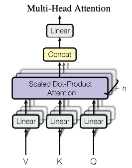
The authors of the paper found that instead of computing attention once using the full embedding size, it was beneficial to project the query, key and value \(h\) times and use those projections to compute the attention, concatenate them together and then again project the concatenated result. The figure below is from the paper that shows how MHA works.

The formula for computing MHA is as follows:

\[MultiHeadAttention(Q, K, V) = Concat(head_1, head_2, ... head_h)W^o \\ head_i = Attention(QW^Q_i, KW^K_i, VW^V_i)\]

We’ll go over step by step to understand each of the concept. For this explanation again, I’ll ignore batch dimension and focus on one sequence only.

Let’s imagine we have a sequence with 3 tokens and each token has 4 dimensional embeddings. The authors also refer to embedding dimension as \(d_{model}\). I’ll just refer to it as embed_dim.

\[input = \begin{bmatrix} how & 1 & 10 & 100 & 1000\\ are & 2 & 20 & 200 & 2000\\ you & 3 & 30 & 300 & 4000 \end{bmatrix}_{3 \times 4}\]

And as mentioned above, we have \(Query = Key = Value = input\) in case of self-attention.

Step 1: Linearly project Query, Key and Value \(h\) times

As shown in the formula, we first need to calculate the output of each head. Let’s consider we have 2 heads (n_heads). Note that the embed_dim must be divisible by n_heads.

Each head will project the Query, Key and Value into embed_dim / n_heads i.e. 4/2 = 2 dimensions. I’ll refer to this as head_dim. This projection is done via a Linear layer where in_features = embed_dim, out_features=head_dim.

Let’s assume that after projection Head 1 and Head 2 produces the following. I’ve used the same value as original embeddings for the sake of explanation.

\[Q_1,K_1,V_1 = \begin{bmatrix} how & 1 & 10\\ are & 2 & 20\\ you & 3 & 30 \end{bmatrix}_{3 \times 2} Q_2,K_2,V_2 = \begin{bmatrix} how & 100 & 1000\\ are & 200 & 2000\\ you & 300 & 4000 \end{bmatrix}_{3 \times 2}\]

Step 2: Compute Attention for each head

Now we compute the attention for each of the heads using the respective Query, Key and Values.

\[head_1 = Attention(Q_1, K_1, V_1) \\ head_2 = Attention(Q_2, K_2, V_2)\]

We’ll have an output something like this. Again for the sake of explanation, let’s assume that 0.1 is added to each value by \(head_1\) and 0.2 by \(head_2\) when computing attention.

\[head_1 = \begin{bmatrix} how & 1.1 & 10.1\\ are & 2.1 & 20.1\\ you & 3.1 & 30.1 \end{bmatrix}_{3 \times 2} head_2 = \begin{bmatrix} how & 100.2 & 1000.2\\ are & 200.2 & 2000.2\\ you & 300.2 & 4000.2 \end{bmatrix}_{3 \times 2}\]

Step 3: Concatenate head outputs

As shown in the formulat, we need to concat the outputs of each head. Also note the shape after concatenation, which is same as the original embedding.

\[input = \begin{bmatrix} how & 1.1 & 10.1 & 100.2 & 1000.2\\ are & 2.1 & 20.1 & 200.2 & 2000.2\\ you & 3.1 & 30.1 & 300.2 & 4000.2 \end{bmatrix}_{3 \times 4}\]

Step 4: Final projection

We again project the concatenated output with a Linear layer. For this layer, the weights is of shape <embed_dim, embed_dim> i.e. in_features = embed_dim, out_features=embed_dim because we want the output of MHA to have same embedding dimension as the input.

After the final projection, MHA is done!

Naive Implementation

Let’s implement MHA using the approach mentioned in the paper where there are \(h\) different heads and each head has its own Linear layers for projecting Query, Key and Value.

class AttentionBlock(torch.nn.Module):
    def __init__(self, input_dim: int, output_dim: int, bias=False):
        super().__init__()
        # Linear layers to project Query, Key and Value 
        self.W_q = torch.nn.Linear(input_dim, output_dim, bias=bias)
        self.W_k = torch.nn.Linear(input_dim, output_dim, bias=bias)
        self.W_v = torch.nn.Linear(input_dim, output_dim, bias=bias)

    def forward(self, query, key, value):
        # project Q, K, V
        q_logits = self.W_q(query)
        k_logits = self.W_k(key)
        v_logits = self.W_v(value)

        # apply scaled dot product attention on projected values
        attn, weights = my_scaled_dot_product_attention(q_logits, k_logits, v_logits)
        return attn, weights

class MyMultiheadAttention(torch.nn.Module):
    def __init__(self, embed_dim: int, n_heads: int, projection_bias=False):
        super().__init__()
        assert embed_dim % n_heads == 0, "embed_dim must be divisible by n_heads"
        self.embed_dim = embed_dim
        self.n_heads = n_heads
        head_embed_dim = self.embed_dim // n_heads
        # for each head, create an attention block
        self.head_blocks = torch.nn.ModuleList([AttentionBlock(input_dim=embed_dim, output_dim=head_embed_dim, bias=projection_bias) for i in range(self.n_heads)])
        # final projection of MHA
        self.projection = torch.nn.Linear(embed_dim, embed_dim, bias=projection_bias)


    def forward(self, query, key, value):
        # these lists are to store output of each head
        attns_list = []
        attn_weights_list = []

        # for every head pass the original query, key, value
        for head in self.head_blocks:
            attn, attn_weights = head(query, key, value)
            attns_list.append(attn)
            attn_weights_list.append(attn_weights)

        # concatenate attention outputs and take average of attention weights
        attns, attn_weights = torch.cat(attns_list, dim=2), torch.stack(attn_weights_list).mean(dim=0)
        # shape: (bs, seq_len, embed_dim), attn_weights: (bs, seq_len, seq_len)
        return self.projection(attns), attn_weights

In the code above we defined a class AttentionBlock which encapsulates the calcuations done by each head. Query, Key and Values are projected independently using 3 different linear layers and then scaled-dot product attention is calculated. Note that in the paper, when projecting they do not add bias but I’ve seen implementations that also add bias. That is why there is a parameter called projection_bias. If we set that to false then it is exactly the same as mentioned in the formula.

MyMultiheadAttention is the class that implements Multi-Head Attention. Here we make sure that embed_dim is divisible by n_heads and then we create AttentionBlock for each head. In the forward method, we loop through each head and then compute the attention. We save both the attention output and the weights in a list. We concatenate the attention outputs using torch.cat(attns_list, dim=2). Since we get multiple attention weights from each head, here I’ve just averaged the attention weights torch.stack(attn_weights_list).mean(dim=0).

Finally we project the attention outputs using self.projection(attns) and return.

This is all there is to it. We can implement this in a bit more efficient way by eliminating the loop over each head. But before we do that let’s use our implementation on a concrete task.

Usage: Text Classification

Let’s build a text classification model using our implementation of MHA and Pytorch’s implementation and compare the performance.

import datasets
from transformers import AutoTokenizer

original_tokenizer = AutoTokenizer.from_pretrained("sentence-transformers/all-MiniLM-L6-v2")


news_ds = datasets.load_dataset("SetFit/bbc-news", split="train")
# train a new tokenizer with limited vocab size for demo
tokenizer = original_tokenizer.train_new_from_iterator(news_ds['text'], vocab_size=1000)

To quickly get started, I’ve loaded a pre-trained tokenizer from HuggingFace hub and a dataset as well. This dataset contains news articles and there are 5 classes: tech, business, sports, entertainment, politics.

To keep things small, I created a new tokenizer with same config as original_tokenizer but with vocabulary size of just 1000. Original tokenizer has vocab size of 30,522 which results in large amount of data in Embedding layer. For this purpose vocab size of 1000 is just fine and we can train our models quickly in CPU as well.

Then we tokenize our dataset and split it into train and test set.

def tokenize(batch):
    return tokenizer(batch['text'], truncation=True)

ds = news_ds.map(tokenize, batched=True).select_columns(['label', 'input_ids', 'text']).train_test_split()

class_id_to_class = {
    0: "tech",
    1: "business",
    2: "sports",
    3: "entertainment",
    4: "politics",
}
num_classes = len(class_id_to_class)

Next, let’s create our text-classification model. The model needs few parameters like vocab_size, embed_dim, num_classes and mha. Since we’ll compare multiple implementations of MHA, we’ll accept this as a parameter when initializing. Note that I’ve implemented a very simple model here and the goal is not to get the best classifier but a working one to compare our MHA implementation.

class TextClassifier(torch.nn.Module):
    def __init__(self, vocab_size: int, embed_dim: int, num_classes: int, mha: torch.nn.Module):
        super().__init__()
        self.embedding = torch.nn.Embedding(num_embeddings=vocab_size, embedding_dim=embed_dim, padding_idx=0)
        self.mha = mha
        self.fc1 = torch.nn.Linear(in_features=embed_dim, out_features=128)
        self.relu = torch.nn.ReLU()
        self.final = torch.nn.Linear(in_features=128, out_features=num_classes)

    def forward(self, input_ids: torch.Tensor, **kwargs):
        # inputs: (bs, seq_len)
        # embeddings: (bs, seq_len, embed_dim)
        embeddings = self.get_embeddings(input_ids)
        attn, attn_weights = self.get_attention(embeddings, embeddings, embeddings)
        
        # take the first token's embeddings i.e. embeddings of CLS token
        # cls_token_embeddings: (bs, embed_dim)
        cls_token_embeddings = attn[:, 0, :] 
        return self.final(self.relu(self.fc1(cls_token_embeddings)))
    
    def get_embeddings(self, input_ids):
        return self.embedding(input_ids)
    
    def get_attention(self, query, key, value):
        attn, attn_weights = self.mha(query, key, value)
        return attn, attn_weights

n_heads = 8
embed_dim = 64
vocab_size = tokenizer.vocab_size
torch_mha = torch.nn.MultiheadAttention(embed_dim=embed_dim, num_heads=n_heads, batch_first=True)
my_mha = MyMultiheadAttention(embed_dim=embed_dim, n_heads=n_heads, projection_bias=True)
torch_classifier = TextClassifier(vocab_size=tokenizer.vocab_size, embed_dim=embed_dim, num_classes=num_classes, mha=torch_mha)
my_classifier = TextClassifier(vocab_size=tokenizer.vocab_size, embed_dim=embed_dim, num_classes=num_classes, mha=my_mha)

Here we have two different classifiers using Pytorch’s implementation vs the one we implemented. Both of them have 8 heads and the embed_dim is 64. If our implementation is correct then both of these models should have almost the same accuracy.

Next, we’ll create a train function with the following signature train(model: torch.nn.Module, train_dl, val_dl, epochs=10) -> list[tuple[float, float]]. This function will train the model and return a list of pairs of numbers indicating train loss and test loss for each epoch. Note that I was running this in CPU so the training loop code does not consider moving tensors/models to GPU.

Click to expand training loop code

from torch.utils.data import DataLoader
import time

def collate_fn(batch):
    labels = []
    input_ids = []
    for row in batch:
        labels.append(row['label'])
        input_ids.append(torch.LongTensor(row['input_ids']))

    input_ids = torch.nn.utils.rnn.pad_sequence(input_ids, batch_first=True, padding_value=0)
    labels = torch.LongTensor(labels)
    input_ids = torch.Tensor(input_ids)
    return {"labels": labels, "input_ids": input_ids}

train_dl = test_dl = DataLoader(ds['train'], shuffle=True, batch_size=32, collate_fn=collate_fn)
test_dl = DataLoader(ds['test'], shuffle=False, batch_size=32, collate_fn=collate_fn)

def train(model: torch.nn.Module, train_dl, val_dl, epochs=10) -> list[tuple[float, float]]:
    optim = torch.optim.AdamW(model.parameters(), lr=1e-3)
    loss_fn = torch.nn.CrossEntropyLoss()
    losses = []
    train_start = time.time()
    for epoch in range(epochs):
        epoch_start = time.time()
        train_loss = 0.0
        model.train()
        for batch in train_dl:
            optim.zero_grad()
            logits = model(**batch)
            loss = loss_fn(logits, batch['labels'])
            loss.backward()
            optim.step()
            train_loss += loss.item() * batch['labels'].size(0)

        train_loss /= len(train_dl.dataset)

        model.eval()
        val_loss = 0.0
        val_accuracy = 0.0
        with torch.no_grad():
            for batch in val_dl:
                logits = model(**batch)
                loss = loss_fn(logits, batch['labels'])
                val_loss += loss.item() * batch['labels'].size(0)
                val_accuracy += (logits.argmax(dim=1) == batch['labels']).sum()

        val_loss /= len(val_dl.dataset)
        val_accuracy /= len(val_dl.dataset)
        log_steps = max(1, int(0.2 * epochs))

        losses.append((train_loss, val_loss))
        if epoch % log_steps == 0 or epoch == epochs - 1:
            epoch_duartion = time.time() - epoch_start
            print(f'Epoch {epoch+1}/{epochs}, Training Loss: {train_loss:.4f}, Validation Loss: {val_loss:.4f}, Validation Accuracy: {val_accuracy:.4f}. Epoch Duration: {epoch_duartion:.1f} seconds')

    train_duration = time.time() - train_start
    print(f"Training finished. Took {train_duration:.1f} seconds")

    return losses

Let’s also quickly check the number of parameters of our models.

def get_model_param_count(model):
    return sum(t.numel() for t in model.parameters())

print(f"My classifier params: {get_model_param_count(my_classifier):,}")
print(f"Torch classifier params: {get_model_param_count(torch_classifier):,}")

# My classifier params: 89,605
# Torch classifier params: 89,605

Now we are ready to train!

torch_losses = train(torch_classifier, train_dl, test_dl, epochs=10)
my_losses = train(my_classifier, train_dl, test_dl, epochs=10)

From the logs, torch_classifier took 155 seconds to train with each epoch taking about 15 seconds. my_classifier however took 218 seconds and each epoch taking about 21 seconds. Clearly our implementation of MHA is not as fast as Pytorch.

The accuracy on test set is also very similar. At the last epoch, torch_classifier had 0.87 accuracy and my_classifier had 0.876. So even though our implementation is slower, it is doing its job. Here is a full output of classification_report.

My Classifier
              precision    recall  f1-score   support

           0       0.90      0.81      0.85        53
           1       0.85      0.90      0.87        69
           2       0.92      0.96      0.94        74
           3       0.88      0.79      0.83        57
           4       0.83      0.89      0.86        54

    accuracy                           0.88       307
   macro avg       0.88      0.87      0.87       307
weighted avg       0.88      0.88      0.88       307

Torch Classifier
              precision    recall  f1-score   support

           0       0.92      0.64      0.76        53
           1       0.86      0.87      0.86        69
           2       0.96      0.96      0.96        74
           3       0.82      0.93      0.87        57
           4       0.82      0.93      0.87        54

    accuracy                           0.87       307
   macro avg       0.87      0.87      0.86       307
weighted avg       0.88      0.87      0.87       307

Code to produce this report is below if you want to take a look.

Click to expand

import toolz

def predict(texts, model, bs=32):
    output_dfs = []
    for batch in toolz.partition_all(bs, texts):
        inputs = tokenizer(batch, return_tensors="pt", padding=True, truncation=True)
        with torch.no_grad():
            class_probs = torch.softmax(model(**inputs), dim=1).numpy()
            pred_classes = class_probs.argmax(axis=1)
            col_names = [f"class_{i}_prob" for i in range(class_probs.shape[-1])]
            df = pd.DataFrame(class_probs, columns=col_names)
            df['pred_class'] = pred_classes
            df['pred_class_name'] = df['pred_class'].map(class_id_to_class)
            output_dfs.append(df)

    return pd.concat(output_dfs)

my_preds_df = predict(ds['test']['text'], my_classifier)
my_preds_df['model'] = 'My Model'
my_preds_df['actual_class'] = ds['test']['label']
torch_preds_df = predict(ds['test']['text'], torch_classifier)
torch_preds_df['model'] = 'Torch Model'
torch_preds_df['actual_class'] = ds['test']['label']

from sklearn.metrics import classification_report

print("My Classifier")
print(classification_report(my_preds_df['actual_class'], my_preds_df['pred_class']))

print("Torch Classifier")
print(classification_report(torch_preds_df['actual_class'], torch_preds_df['pred_class']))

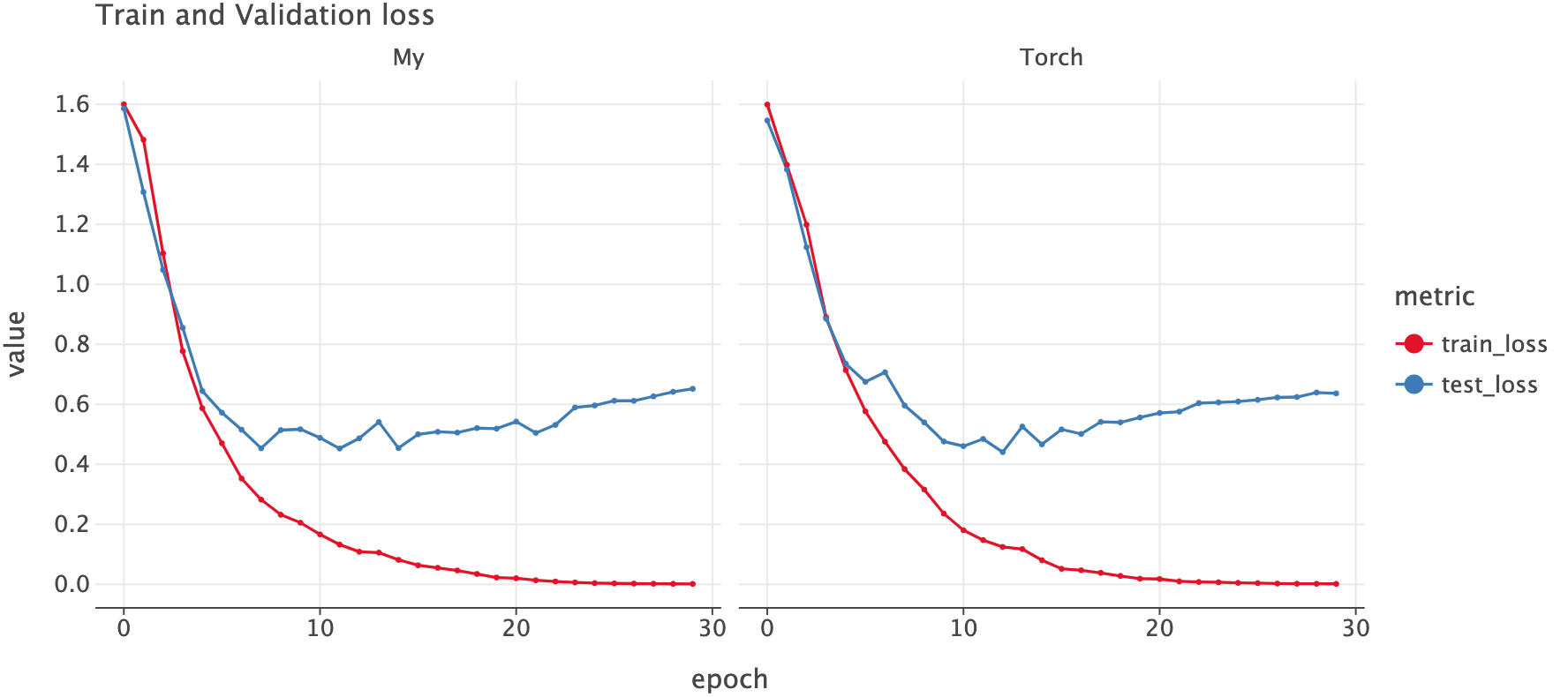
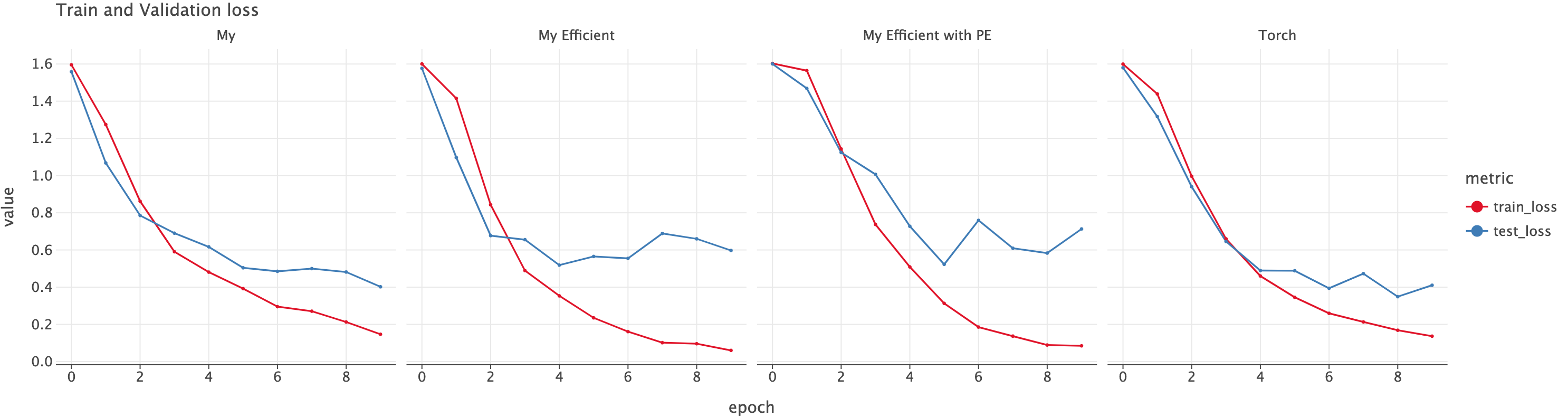
Let’s plot the loss for both of these models. We see similar pattern for both the models.

Click to expand

def get_losses_as_df(losses_name_pairs: list[tuple[str, tuple[float, float]]]):
    dfs = []
    for model_name, losses in losses_name_pairs:
        df = pd.DataFrame(losses, columns=['train_loss', 'test_loss']).reset_index().rename(columns={"index": "epoch"})
        df['model'] = model_name
        dfs.append(df)
    return pd.concat(dfs)

def plot_losses(loss_df):
    df = loss_df.melt(id_vars=['model', 'epoch'], var_name='metric')
    return ggplot(df, aes('epoch', 'value', color='metric')) + geom_line() + geom_point(size=1.5) + facet_grid('model') + labs(title="Train and Validation loss")


plot_losses(get_losses_as_df([("My", my_losses), ("Torch", torch_losses)]))

Efficient MHA Implementation

In our first implementation, we looped through each head which independently projected the query, key and value. There were two heads, so the query was projected 2 times by two heads and same for key and value. In total there were 6 “projections” happening. However we can reduce it to just 3 projection operations.

Let’s focus on projection of Query by the two heads. Let’s say we have the following as our original input.

\[input = Q = \begin{bmatrix} how & 1 & 10 & 100 & 1000\\ are & 2 & 20 & 200 & 2000\\ you & 3 & 30 & 300 & 3000 \end{bmatrix}_{3 \times 4}\]

Since there are two heads, the projection weight of these two heads will be of shape \(2 \times 4\) i.e <out_features, in_features>. Let’s assume we have the following weights.

\[W_1 = \begin{bmatrix} 10 & 0 & 0 & 0\\ 0 & 10 & 0 & 0 \end{bmatrix}_{2 \times 4} \\ W_2 = \begin{bmatrix} 20 & 0 & 0 & 0\\ 0 & 20 & 0 & 0 \end{bmatrix}_{2 \times 4}\]

Now each head will project the Query

\[QW_1^T = \begin{bmatrix} how & 1 & 10 & 100 & 1000\\ are & 2 & 20 & 200 & 2000\\ you & 3 & 30 & 300 & 3000 \end{bmatrix}_{3 \times 4} \begin{bmatrix} 10 & 0 \\ 0 & 10 \\ 0 & 0 \\ 0 & 0 \\ \end{bmatrix}_{4 \times 2} \\ = \begin{bmatrix} 10 & 100\\ 20 & 200\\ 30 & 300 \end{bmatrix}_{3 \times 2} \\ QW_1^T = \begin{bmatrix} how & 1 & 10 & 100 & 1000\\ are & 2 & 20 & 200 & 2000\\ you & 3 & 30 & 300 & 3000 \end{bmatrix}_{3 \times 4} \begin{bmatrix} 20 & 0 \\ 0 & 20 \\ 0 & 0 \\ 0 & 0 \\ \end{bmatrix}_{4 \times 2} \\ = \begin{bmatrix} 20 & 200\\ 40 & 400\\ 60 & 600 \end{bmatrix}_{3 \times 2}\]

So we’ve obtained the projections from both heads for query by performing two individual projections. However, the projection weight can be stacked together so that we can obtain the projection in one matrix multiplication.

\[Q = \begin{bmatrix} how & 1 & 10 & 100 & 1000\\ are & 2 & 20 & 200 & 2000\\ you & 3 & 30 & 300 & 3000 \end{bmatrix}_{3 \times 4} W = \begin{bmatrix} 10 & 0 & 0 & 0\\ 0 & 10 & 0 & 0\\ 20 & 0 & 0 & 0\\ 0 & 20 & 0 & 0 \end{bmatrix}_{4 \times 4} \\ QW^T = \begin{bmatrix} how & 1 & 10 & 100 & 1000\\ are & 2 & 20 & 200 & 2000\\ you & 3 & 30 & 300 & 3000 \end{bmatrix}_{3 \times 4} \begin{bmatrix} 10 & 0 & 20 & 0\\ 0 & 10 & 0 & 20\\ 0 & 0 & 0 & 0\\ 0 & 0 & 0 & 0\\ \end{bmatrix}_{4 \times 4} \\ = \begin{bmatrix} 10 & 100 & 20 & 200\\ 20 & 200 & 40 & 400\\ 30 & 300 & 60 & 600 \end{bmatrix}_{3 \times 4}\]

As you can see we obtained the same value with just one matrix multiplication compared with two individual ones. The first two columns have same value as the projection of 1st head and the last two columns have same value as projection of second head.

So now we know that we can do the projection just once there by eliminating the for loop. However, we cannot use this projection and pass it to the attention function. Remember that this is a mult-head attention so attention will be calculated using different portion of the data. So we need to reshape this output a bit.

We have batch_size = 1, n_heads = 2 and projection shape = <3, 4>. We know the for head 1 and head 2 the projection should be of shape <3, 2>. So we reshape the data as follows.

1. projection.view(batch_size, seq_len, n_heads, head_embed_dim).

\[\begin{bmatrix} Batch & Token & Head & Vector\\ 1 & how & 1 & [10, 100] \\ 1 & how & 2 & [20, 200] \\ 1 & are & 1 & [20, 200] \\ 1 & are & 2 & [40, 400] \\ 1 & you & 1 & [30, 300] \\ 1 & you & 2 & [60, 600] \end{bmatrix}\]

Since we want to calculate attention per head, we swap token and head using reshaped.transpose(1, 2) resulting in

\[\begin{bmatrix} Batch & Head & Token & Vector\\ 1 & 1 & how & [10, 100]\\ 1 & 1 & are & [20, 200]\\ 1 & 1 & you & [30, 300]\\ 1 & 2 & how & [20, 200]\\ 1 & 2 & are & [40, 400]\\ 1 & 2 & you & [60, 600]\\ \end{bmatrix}\]

Now we have the data laid out in proper format, we can pass this to the scaled dot product attention function.

The attention output will be of shape <batch_size, n_heads, seq_len, head_embed_dim>. But we need the data to have shape of <batch_size, seq_len, embed_dim> before applying the final projection of the MHA layer.

To do this we swap the n_heads, and seq_len using attn.transpose(1, 2).contiguous() so that we have the shape <batch_size, seq_len, n_heads, head_embed_dim. Then we “flatten” the n_heads dimension so that we end up with <batch_size, seq_len, embed_dim> using attn_transposed.view(batch_size, seq_len, embed_dim). We are basically reversing what we did earlier. Check the implementation below.

class MyEfficientMultiHeadAttention(torch.nn.Module):
    def __init__(self, embed_dim: int, n_heads: int, projection_bias=False):
        super().__init__()
        assert embed_dim % n_heads == 0, "embed_dim must be divisible by n_heads"
        self.embed_dim = embed_dim
        self.n_heads = n_heads
        self.head_embed_dim = self.embed_dim // n_heads
        self.W_q = torch.nn.Linear(embed_dim, embed_dim, bias=projection_bias)
        self.W_k = torch.nn.Linear(embed_dim, embed_dim, bias=projection_bias)
        self.W_v = torch.nn.Linear(embed_dim, embed_dim, bias=projection_bias)
        self.projection = torch.nn.Linear(embed_dim, embed_dim, bias=projection_bias)

    def forward(self, query, key, value):
        # shape of query = (bs, seq_len, embed_dim)
        batch_size = query.size(0)

        # linear projection of query, key and value
        q = self.W_q(query)
        k = self.W_k(key)
        v = self.W_v(value)

        # reshape the projected query, key, value
        # to (bs, n_heads, seq_len, head_embed_dim)
        q = self.split_heads(q)
        k = self.split_heads(k)
        v = self.split_heads(v)

        # do scaled dot product attention
        # attn.shape = (bs, n_heads, seq_len, head_embed_dim)
        # attn_weights.shape (bs, n_heads, seq_len, seq_len)
        attn, attn_weights = my_scaled_dot_product_attention(q, k, v)
        # swap the n_heads and seq_len so that we have
        # (bs, seq_len, n_heads, head_embed_dim)
        # call .contiguous() so that view function will work later
        attn = attn.transpose(1, 2).contiguous()
        # "combine" (n_heads, head_embed_dim) matrix as a single "embed_dim" vector
        attn = attn.view(batch_size, -1, self.embed_dim)

        output = self.projection(attn)
        return output, attn_weights.mean(dim=1)

    def split_heads(self, x):
        # x.shape = (bs, seq_len, embed_dim)
        batch_size = x.size(0)
        # first split the embed_dim into (n_heads, head_embed_dim)
        temp =  x.view(batch_size, -1, self.n_heads, self.head_embed_dim)
        # now we swap seq_len and n_heads dimension
         # output shape = (bs, n_heads, seq_len, head_embed_dim)
        return temp.transpose(1, 2)

Now let’s use this implementation and see if we see improvements in training speed.

my_efficient_mha = MyEfficientMultiHeadAttention(embed_dim=embed_dim, n_heads=n_heads, projection_bias=True)
my_efficient_classifier = TextClassifier(vocab_size=tokenizer.vocab_size, embed_dim=embed_dim, num_classes=num_classes, mha=my_efficient_mha)
my_efficient_losses = train(my_efficient_classifier, train_dl, test_dl, epochs=10)

This implementation took 186 seconds to train with about 18.5 seconds per epoch. It is still slower than Pytorch’s implementation (155 seconds) but much quicker than our naive implementation (218 seconds). The accuracy on test set is 0.85 which is also very close to the previous two (~0.87).

Positional Embeddings

One thing you might have noticed is that there is no notion of order of tokens when we compute attention. Every token is attending to every other. This is to say that ‘how are you’ is exactly the same as ‘you how are’ or ‘are you how’. We’ll get the same representation no matter how we order the tokens. This is very similar to Bag-of-words model like TF-IDF.

For example, if we ask the model to predict for the following sentences, we get the same output probabilities since the representation of each of those tokens is exactly the same which in turn means that the representation of both the sentences is also exactly the same!

predict(["how are you", "you how are"], torch_classifier)

	class_0_prob	class_1_prob	class_2_prob	class_3_prob	class_4_prob	pred_class	pred_class_name
0	0.018061	0.564215	0.01021	0.379704	0.027809	1	business
1	0.018061	0.564215	0.01021	0.379704	0.027809	1	business

To give the model some information about the order of tokens, we use something called Positional Embeddings or Encoding. Basically, after we get the embeddings from the Embedding layer, we add positional embeddings (element wise). This will make sure even for same token, the “position-embedded” embedding will have different values because of their position in the sequence.

This post has gotten too long already so you can refer to this Notebook which explains positional embedding. I’ve copied the code from there.

class PositionalEncoding(torch.nn.Module):
    # source: https://uvadlc-notebooks.readthedocs.io/en/latest/tutorial_notebooks/tutorial6/Transformers_and_MHAttention.html#Positional-encoding
    def __init__(self, embed_dim, max_len=256):
        super().__init__()
        # create a matrix of [seq_len, hidden_dim] representing positional encoding for each token in sequence
        pe = torch.zeros(max_len, embed_dim)
        position = torch.arange(0, max_len, dtype=torch.float).unsqueeze(1) # (max_len, 1)
        div_term = torch.exp(torch.arange(0, embed_dim, 2).float() * (-math.log(10000.0) / embed_dim))
        pe[:, 0::2] = torch.sin(position * div_term)
        pe[:, 1::2] = torch.cos(position * div_term)
        pe = pe.unsqueeze(0)
        self.register_buffer('pe', pe, persistent=False)

    def forward(self, x):
        x = x + self.pe[:, :x.size(1)]
        return x
    
class TextClassifierWithPositionalEncoding(TextClassifier):
    def __init__(self, vocab_size: int, embed_dim: int, num_classes: int, mha: Module, max_len: int=256):
        super().__init__(vocab_size, embed_dim, num_classes, mha)
        self.positional_encoding = PositionalEncoding(embed_dim=embed_dim, max_len=max_len)

    def get_embeddings(self, input_ids):
        embeddings = super().get_embeddings(input_ids)
        return self.positional_encoding(embeddings)

Here I’ve subclassed TextClassifier and created a new class TextClassifierWithPositionalEncoding which overloads the get_embeddings method. First we get the token embeddings and then add the positional embeddings to the token embeddings. This will now be used by the MHA layer.

Let’s train the model with Positional Embedding and see what we get.

my_efficient_mha2 = MyEfficientMultiHeadAttention(embed_dim=embed_dim, n_heads=n_heads, projection_bias=True)
my_efficient_classifier_with_pe = TextClassifierWithPositionalEncoding(vocab_size=tokenizer.vocab_size, embed_dim=embed_dim, num_classes=num_classes, mha=my_efficient_mha2, max_len=tokenizer.model_max_length)
my_efficient_losses_with_pe = train(my_efficient_classifier_with_pe, train_dl, test_dl, epochs=10)

It took 195 seconds with each epoch taking about 19 seconds. The accuracy in the validation set is 0.81 which is pretty low compared to others (0.85 and 0.87).

Once again, here is the loss over epoch for all different implementations.

Let’s see if Position Embedding did change something. Now if we ask the classifier to predict using predict(["how are you", "you how are"], my_efficient_classifier_with_pe)

	class_0_prob	class_1_prob	class_2_prob	class_3_prob	class_4_prob	pred_class	pred_class_name
0	0.037759	0.028393	0.066061	0.488044	0.379744	3	entertainment
1	0.031583	0.022696	0.055122	0.538267	0.352332	3	entertainment

We see that the probabilities are different since now both sentences have different representations. Model without using Positional Embedding predicted exactly the same probabilities for both sentences.

Before we conclude, let’s visualize the attention weights as well. Below I’ve used this sentence as input: can you can that. The first “can” is a verb asking if someone can do something e.g. “can you do that?” and the second “can” is a verb meaning to preserve something in a can or a jar. This is a short and confusing sentence so let’s see how the attention weights look like.

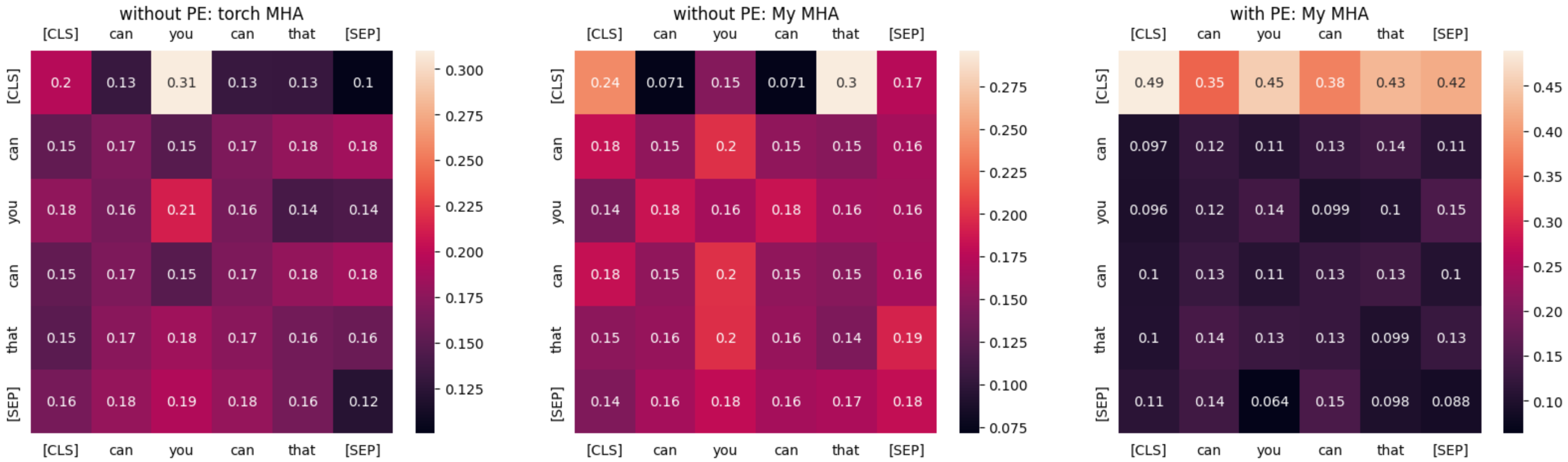
For the first two models that do not use Positonal Embedding, take a look at the rows of the word ‘can’. Both occurrence of this word has exactly the same attention weight with other tokens. But when we introduce Positional Embedding, the first ‘can’ has highest attention weight with the word ‘that’ and the second occurrence of ‘can’ has almost equal attention to the first ‘can’, itself and ‘that’.

Since the model was trained to classify with only 80K parameters with very small dataset about news, the attention weights might not make sense so I suggest not to decode the numbers too much. My intention here was just to show that using Positional Embeddings impact the outputs.

You can use the code below to generate the plot shown above.

Click to expand the code

import seaborn as sns
import matplotlib.pyplot as plt

def visualize_attention_weights(model, text, tokenizer, ax):
    inputs = tokenizer(text, return_tensors="pt", truncation=True)
    with torch.no_grad():
        embeddings = model.get_embeddings(inputs['input_ids'])
        attn_weights = model.get_attention(embeddings, embeddings, embeddings)[1].squeeze()

    tokens = tokenizer.convert_ids_to_tokens(inputs['input_ids'].squeeze())
    df = pd.DataFrame(attn_weights, columns=tokens, index=tokens)
    return sns.heatmap(df, annot=True, ax=ax)
    
# "Can you can that?" -> First can is a verb, second can is a verb: to preserve something in a Can
fig, axes = plt.subplots(1, 3, figsize=(20, 5), sharey=False)
for i, (model_name, model) in enumerate([("without PE: torch MHA", torch_classifier), ("without PE: My MHA", my_classifier), ("with PE: My MHA", my_efficient_classifier_with_pe)]):
    axes[i] = visualize_attention_weights(model, text="can you can that", tokenizer=tokenizer, ax=axes[i])
    axes[i].set_title(model_name)
    axes[i].tick_params(labeltop=True, bottom=False, left=False)

Conclusion

In this post, we implemented everything we need to use Multi-Head Attention (except masking). To summarize

• The dot product of the Query and Key determines the weight assigned to the corresponding Value vector.
• Multi-Head Attention uses multiple heads, each focusing on different parts of the projected Query, Key, and Value vectors, allowing the model to capture various patterns in the data.
• We efficiently implemented Multi-Head Attention to optimize performance.
• Why Positional Embeddings are needed and how they impact the learned behaviour

I hope this post was useful. Please let me know if there are any mistakes in this post.

This article is Part 1 in a 5-Part Understanding Transformers Architecture.

• Part 1 - > Multi-Head Attention From Scratch
• Part 2 - Masking in Transformer Encoder/Decoder Models
• Part 3 - Implementing Transformer Encoder Layer From Scratch
• Part 4 - Implementing Transformer Decoder Layer From Scratch
• Part 5 - Decoding strategies in Decoder models (LLMs)